Primer I: Quick Start
This primer will lead you through the steps to make a simple plot (maybe your first!) with R, a free and open-source software environment for statistical computing and graphics. You can read more about it here https://www.r-project.org.
Our end goal is to get you looking at a screen like this:
Packages
The version of R that you just downloaded is considered base R, which provides you with good but basic statistical computing and graphics powers. For analytical and graphical super-powers, you’ll need to install add-on packages, which are user-written, to extend/expand your R capabilities.
R packages can live in one of two places:
-
They may be carefully curated by CRAN (https://cran.r-project.org/). CRAN stands for the “Comprehensive R Archive Network”, which involves a thorough submission and review process for R packages. Packages that go through this process and are accepted by CRAN are easy to install from your R console using:
```{r}
install.packages("name_of_package")
```
In your R console, let’s install the remotes package:
```{r} install.packages("remotes") ``` -
Alternatively, they may be available via GitHub. Sometimes, a package is available in both places. Many R packages use GitHub for development, and submit new versions occasionally to CRAN. CRAN packages are often considered to be ‘stable’ versions. Packages from GitHub are considered to be the in-development versions.
To download an R package from GitHub, you first need to install the remotes package from CRAN, which we just did! Then you can run this code in your R console:
```{r}
library(remotes)                   # load the remotes package
install_github("username/repo")    # use a function from remotes
```
The
install_github()statement is a function, and the part in quotes ("username/repo") refers to URL for the R package on GitHub. For example, we made a package for this book that you can find at https://github.com/dspatterns/dspatterns. To install that package, run the following code in your R console:```{r} library(remotes) install_github("dspatterns/dspatterns") ```
Place your cursor in the console again (where you last typed x and [4] printed on the screen). You can use the first method to install the following packages directly from CRAN, all of which we will use:
Mind your use of quotes carefully with packages.
- To install a package, you put the name of the package in quotes as in
install.packages("name_of_package"). - To use an already installed package, you must load it first, as in
library(name_of_package). You only need to do this once per RStudio session.
Two good rules of thumb when working with packages in R:
Install packages once per workstation/machine. Always use the console when using
install.packages().Load packages once per work session. Each
library()call typically goes on its own line when we put our code in an R script or Quarto document.
You can download all of these at once, too:
install.packages(c("dplyr", "ggplot2", "babynames"), dependencies = TRUE)We should formally introduce the combine command, c(), used above. You will use this often- any time you want to combine things into a vector.
c("hello", "my", "name", "is", "alison")[1] "hello" "my" "name" "is" "alison"c(1:3, 20, 50)[1] 1 2 3 20 50R is case-sensitive, so ?dplyr works but ?Dplyr will not. Likewise, a variable called A is different from a.
Open a new R script in RStudio by going to File --> New File --> R Script. For this first foray into R, we’ll give you the code, so sit back and relax—feel free to copy and paste our code in with some small tweaks.
First we’ll load the packages:
```{r}
library(babynames)  # contains the actual data
library(dplyr)      # for manipulating data
library(ggplot2)    # for plotting data
```
and in the next section, we’ll begin using some functions.
Functions
Here are some critical commands to obtain a high-level overview of your freshly read dataset in R. We’ll call it saying ‘hello’ to your dataset:
glimpse(babynames)Rows: 1,924,665
Columns: 5
$ year <dbl> 1880, 1880, 1880, 1880, 1880, 1880, 1880, 1880, 1880, 1880, 1880,…
$ sex <chr> "F", "F", "F", "F", "F", "F", "F", "F", "F", "F", "F", "F", "F", …
$ name <chr> "Mary", "Anna", "Emma", "Elizabeth", "Minnie", "Margaret", "Ida",…
$ n <int> 7065, 2604, 2003, 1939, 1746, 1578, 1472, 1414, 1320, 1288, 1258,…
$ prop <dbl> 0.07238359, 0.02667896, 0.02052149, 0.01986579, 0.01788843, 0.016…head(babynames)# A tibble: 6 × 5
year sex name n prop
<dbl> <chr> <chr> <int> <dbl>
1 1880 F Mary 7065 0.0724
2 1880 F Anna 2604 0.0267
3 1880 F Emma 2003 0.0205
4 1880 F Elizabeth 1939 0.0199
5 1880 F Minnie 1746 0.0179
6 1880 F Margaret 1578 0.0162tail(babynames)# A tibble: 6 × 5
year sex name n prop
<dbl> <chr> <chr> <int> <dbl>
1 2017 M Zyhier 5 0.00000255
2 2017 M Zykai 5 0.00000255
3 2017 M Zykeem 5 0.00000255
4 2017 M Zylin 5 0.00000255
5 2017 M Zylis 5 0.00000255
6 2017 M Zyrie 5 0.00000255names(babynames)[1] "year" "sex" "name" "n" "prop"If you have done the above and produced sane-looking output, you are ready for the next step. We’ll use the code below to create a new data frame called alison.
The first bit makes a new dataset called
alisonthat is a copy of thebabynamesdataset- the|>tells you we are doing some other stuff to it later.The second bit
filtersourbabynamesto only keep rows where thenameis equal to “Alison” (read==as “exactly equal to”) or “Allison” (read|as “or”.)The third bit applies another
filterto keep only those wheresexis female.
Let’s check out the data (in two different ways):
alison# A tibble: 218 × 5
year sex name n prop
<dbl> <chr> <chr> <int> <dbl>
1 1905 F Alison 7 0.0000226
2 1907 F Alison 5 0.0000148
3 1908 F Allison 6 0.0000169
4 1910 F Alison 5 0.0000119
5 1910 F Allison 5 0.0000119
6 1911 F Allison 9 0.0000204
7 1912 F Allison 12 0.0000204
8 1912 F Alison 9 0.0000153
9 1913 F Alison 12 0.0000183
10 1913 F Allison 7 0.0000107
# ℹ 208 more rowsglimpse(alison)Rows: 218
Columns: 5
$ year <dbl> 1905, 1907, 1908, 1910, 1910, 1911, 1912, 1912, 1913, 1913, 1914,…
$ sex <chr> "F", "F", "F", "F", "F", "F", "F", "F", "F", "F", "F", "F", "F", …
$ name <chr> "Alison", "Alison", "Allison", "Alison", "Allison", "Allison", "A…
$ n <int> 7, 5, 6, 5, 5, 9, 12, 9, 12, 7, 22, 11, 16, 13, 24, 15, 20, 15, 3…
$ prop <dbl> 2.259e-05, 1.482e-05, 1.692e-05, 1.192e-05, 1.192e-05, 2.037e-05,…Again, if you have proper-looking output here, move along to plotting the data.
Now if you did this right, you will not see your plot! Because we saved the plot with a name (plot), R just saved the object for you. But check out the top right pane in RStudio again: under Values you should see plot, so it is there, you just have to ask for it. Here’s how:
plot 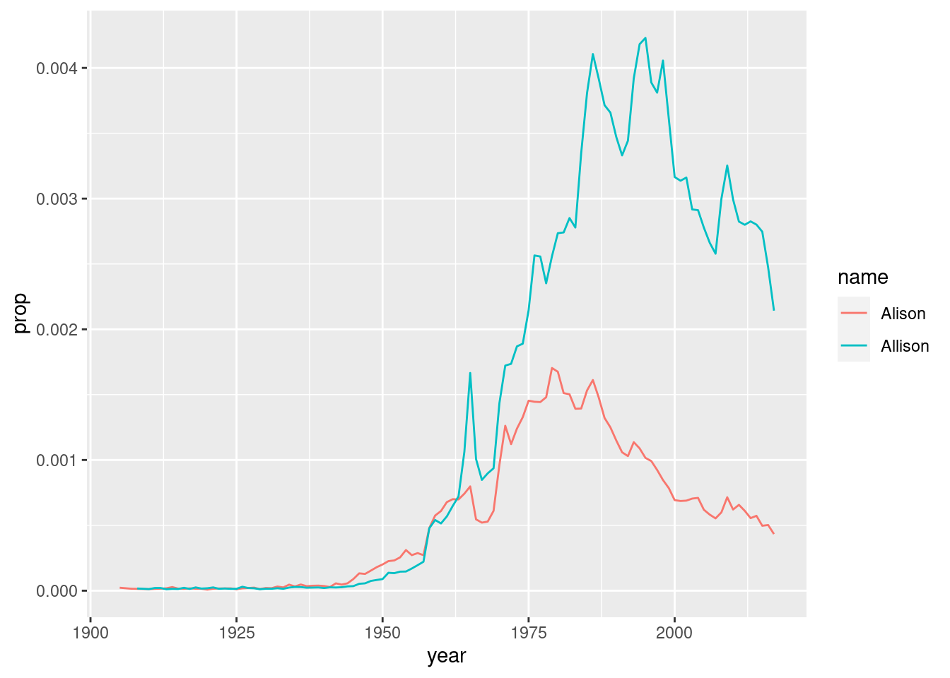
DIY: Make a New Name Plot
Edit the code above to create a new dataset. Pick two names to compare how popular they each are (these could be different spellings of your own name, like I did, but you can choose any two names that are present in the dataset). Make the new plot, changing the name of the first argument alison in ggplot() to the name of your new dataset.