| Write this down as Markdown... | ...get this in HTML form |
|---|---|
|
Plain text |
|
italics and bold |
|
|
|
strikethrough |
|
subscript2 / superscript2 |
|
|
|
inline equation: \(E=mc^2\) |
|
Biggest Heading |
|
Smallest Heading |
|
block quote |
|
|
|
|
Primer II: Quarto
Hello Quarto!
tl;dr: - Quarto is a way to run R code and create a report from a combination of prose and code.
Reporting the results of a data analysis is quite important and is often the deliverable. R has something known as Quarto which is a format for writing code and prose in the same document. The idea for this comes from literate programming, where the mixture of source code for a computer program is intertwined both with an explanation of what the program is doing and also the results of running the program.
There are many advantages of taking this approach for all of your data analysis tasks:
- The explanation of the code is adjacent to the code itself; code comments are like this, but these explanations are more prominent and accessible than source code comments.
- There is no risk of having the code explanation and the code itself dissociated from one another; these two elements are tightly bound.
- A single document contains all of the analysis which is part code and part explanation. It’s self-contained.
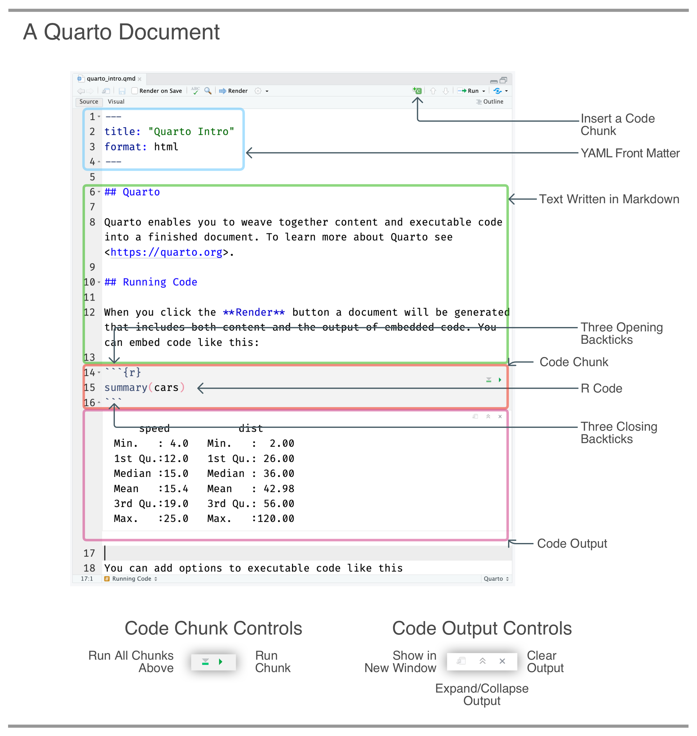
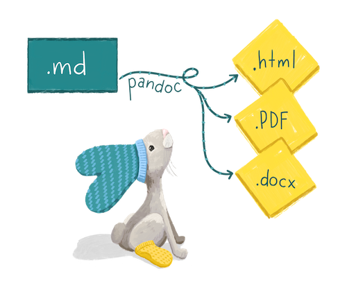
You may or may not be familiar with Markdown, which is a big part of this format. Markdown is a text markup language that translates really well to HTML. It was created as a very simple way for anybody (i.e., non-programmers) to write in an easy-to-read format that could be converted directly into HTML. The following table provides a quick rundown of what typical Markdown looks like before and after rendering to HTML.
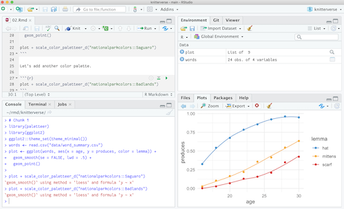
The prose portion of Quarto (i.e., not the R code) is the default text entry type. The R code is run inside code cells, which are marked off areas (with three backticks: ```) in the document. The schematic below shows what an R code cell looks like and what controls are available in Quarto.
Aside from reproducibility, the finished Quarto document can be rendered to a self-contained HTML file, to a Word document, to a various presentation types including Powerpoint, or to a PDF file. There are lots of ways to customize what the rendered document will look like (e.g., hiding code for non-technical audiences, adding HTML display elements, etc.), so, the analysis can double as a deliverable report. This will undoubtedly save you time. If ever the input data should change, the report could be run again and updated, usually with minimal (if any) modification. That’s one of the features of reproducible reporting.
Let’s walk through a simple example of how to use Quarto in RStudio. You probably don’t know any R at this point and that’s perfectly fine. The point of this example is to show some of the mechanics of using the interface to run code and generate an HTML report. The main things we’ll do in this Quarto walkthrough are to fill in the YAML front matter (these are basic rendering instructions), add in two R code cells (displaying a data summary and showing a plot), and adding Markdown text with basic explanations.
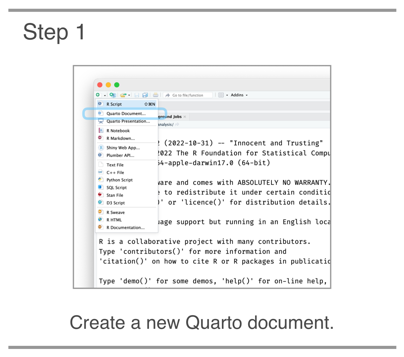 STEP 1. The first thing to do is create a new Quarto document. This is conveniently done through the New File dropdown button (top left of IDE). A new Quarto document is the third choice from the top.
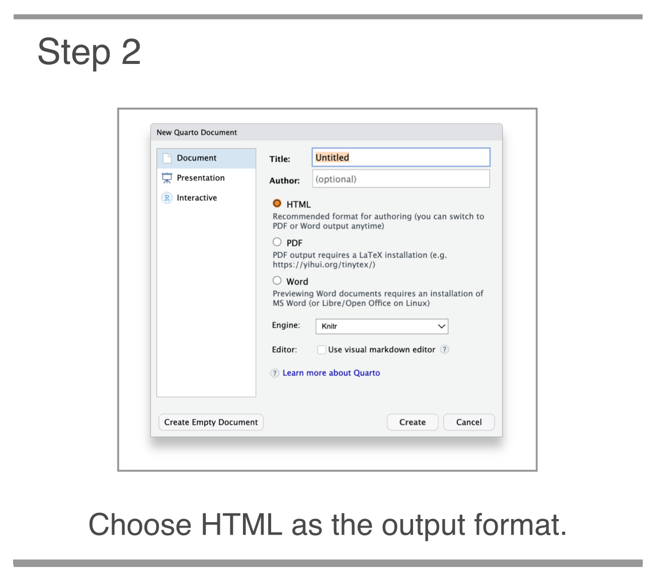
STEP 2. You’ll be presented with a dialog box and some options. The default option of HTML is what we want for this walkthrough, so hit Enter or the OK button. A new, untitled Quarto document will appear in the Source pane (the top-left pane).
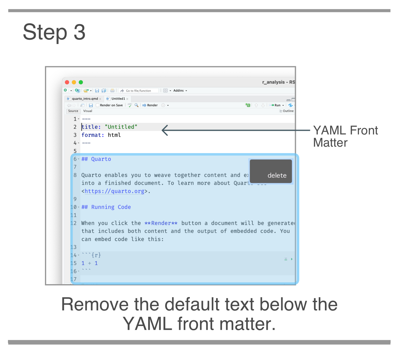
STEP 3. We should delete everything in this default document except for the useful YAML front matter (i.e., the text enclosed by three hyphens). Then save the document as a .qmd file. Saving is necessary before rendering and is generally considered a good practice (though RStudio will always keep your unsaved documents across sessions).
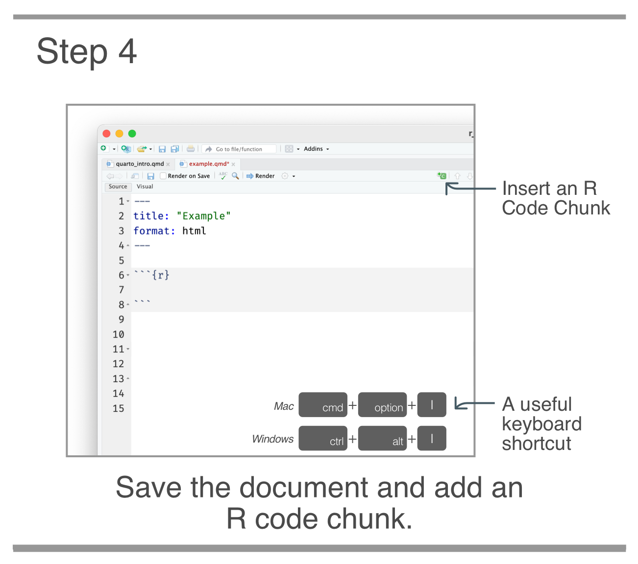
STEP 4. Now, place the insertion point in the document below the YAML and insert an R code cell. This can be done with the handy keyboard shortcut Command + Option + I (Control + Alt + I on Windows). You’ll see a text area enclosed by backticks and the language of the code in curly braces: {r}.
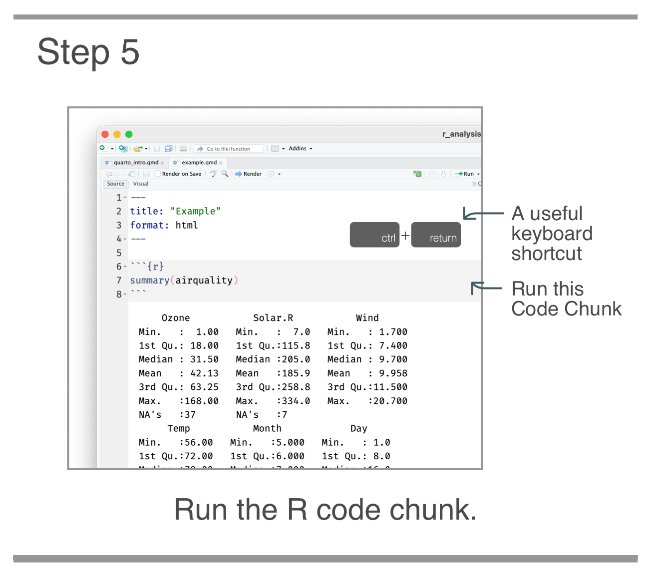
STEP 5. Now we can do some writing of code. Place the insertion point inside the R code cell and type summary(airquality) (this is a built-in R dataset and is always available). Then, run the code in that code cell by pressing the green run button, or, with the keyboard shortcut: Control + Enter. You’ll see a summary of data appear below! Running the code and verifying the output matches expectations is great for practice (although running every code cell is not necessary for rendering the Quarto document).
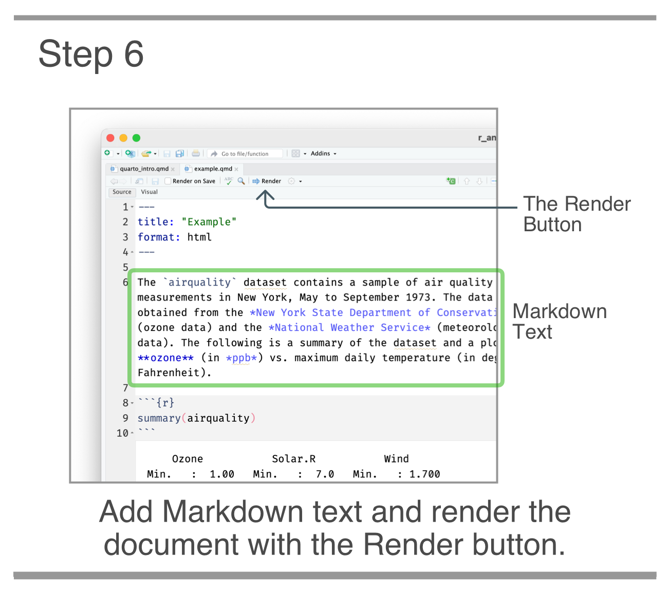
STEP 6. To make this document function as a report, let’s add some text above and below the R code cell. Here is the Markdown text that could be put in above:
The `airquality` dataset contains a sample of air quality measurements in New York, May to September 1973. The data were obtained from the *New York State Department of Conservation* (ozone data) and the *National Weather Service* (meteorological data). The following is a summary of the dataset and a plot of **ozone** (in *ppb*) vs. maximum daily temperature (in degrees Fahrenheit).The Markdown text for below the code cell can be:
For more information on this dataset, use `help(airquality)` in the R console.Inside the IDE, this just looks like plaintext with some highlighting applied when using asterisks or other Markdown elements. Let’s render the document by pressing the Render button that is on the toolbar.
That will produce an HTML document with the same name as the Quarto document (in the directory where the .qmd file was saved) and the process opens a preview window with the HTML report.
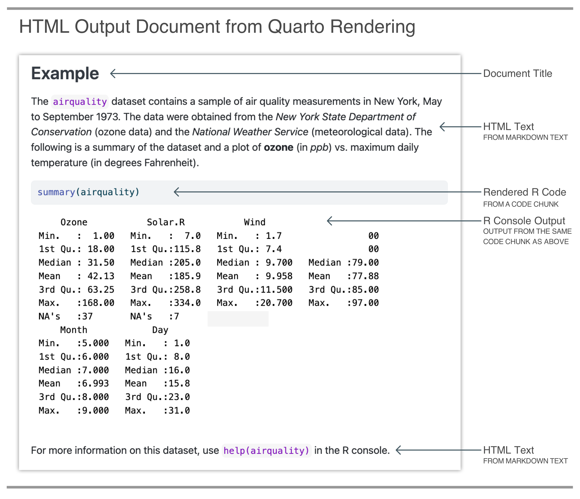
It’s here where you can see that the Markdown elements become things like bold and italicized text. That rendered text appears above and below the code and the outputs, just as it was in the Quarto document. It’s also here where its more apparent that Quarto is indeed useful for working with data and also for creating reports.
More about Quarto
Quarto is open-source software that helps you develop your code and ideas in one reproducible document. It is designed for anyone who uses code to work with data. You can use Quarto at any stage of an analysis project, any time you want to develop code and ideas alongside each other.
Start a Quarto project if you want to:
Save, execute, and explain your code, all in the same place. Develop your code and ideas in one reproducible document.
Transform your code into polished and professional data products—reports, dashboards, websites, slides, even books. Knit plots, tables, and results together with narrative text, and create analyses ready to be shared.
What is a .qmd file?
Every Quarto project starts with a Quarto file that has the extension .qmd.
This particular one analyzes children’s early words, but every .qmd includes the same three basic elements inside:
- A block of metadata at the top, between two fences of
---s. This is written in YAML. - Narrative text, written in Markdown.
- Code cells in gray between two fences of
```, written with R or another programming language.
You can use all three elements to develop your code and ideas in one reproducible document.
How do I create a .qmd file?
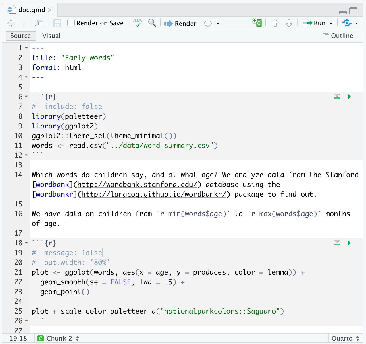
Here is a plain text version of a .qmd document, which you can copy and paste into a new document:
---
title: "Early words"
format: html
---
```{r}
#| include: false
library(paletteer)
library(ggplot2)
ggplot2::theme_set(theme_minimal())
words <- read.csv("../data/word_summary.csv")
```
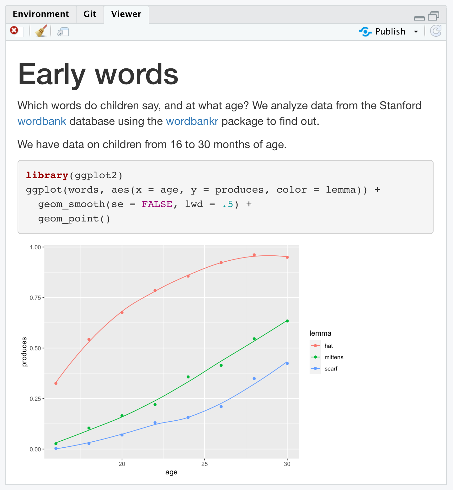
Which words do children say, and at what age? We analyze data from the Stanford [wordbank](http://wordbank.stanford.edu/) database using the [wordbankr](http://langcog.github.io/wordbankr/) package to find out.
We have data on children from `r min(words$age)` to `r max(words$age)` months of age.
```{r}
#| message: false
#| out.width: '80%'
plot <-
ggplot(words, aes(x = age, y = produces, color = lemma)) +
geom_smooth(se = FALSE, lwd = .5) +
geom_point()
plot + scale_color_paletteer_d("nationalparkcolors::Saguaro")
```Quarto helps you create dynamic documents that combine code, rendered output (such as figures), and markdown-formatted text. It was developed by software engineers at Posit, so it works well with the RStudio IDE, which is our IDE of choice for using Quarto with code written in R.
In the rest of this primer, we’ll focus on using Quarto to create .qmd documents that integrate narrative text, code, and its output. While Quarto allows for many different kinds of output, we will use HTML documents. But the possibilities are endless 😃 In fact, this book was also written in Quarto, and its full source is publicly available in the GitHub repository: https://github.com/dspatterns/dspatterns-book.
Developing Code
The code inside your Quarto documents will often start small, then grow as you work. It is totally natural to use your .qmd as a scratchpad to develop code. Many users find that using .qmd files helps them ‘code while thinking’.
Also, .qmd files are designed to be used interactively in RStudio. You can use RStudio to test your code one code cell at a time, which we’ll show now.
Running code cells
If you take everything from the .qmd given above and create a new .qmd in RStudio, you can experiment with running the code. For every gray code cell, you’ll notice a green arrow on the right: 
When you click the run button, the code is evaluated and the output will appear. If you run the second code cell after the first, it also works! This is because RStudio is running your code cells in your global environment, so it finds any objects already assigned.
Results like plots and tables are appear inline in your document. The cool thing about this is that your source .qmd file won’t change on the basis of the output.
Adding new code cells
Now let’s add a new code cell. You can insert code cells in any of three ways:
use the Add Chunk
 button in the editor toolbar
use the keyboard shortcut Ctrl + Alt + I (OS X: Cmd + Option + I)
type
```{r}and```(the symbols are backticks)
Setting up your panes
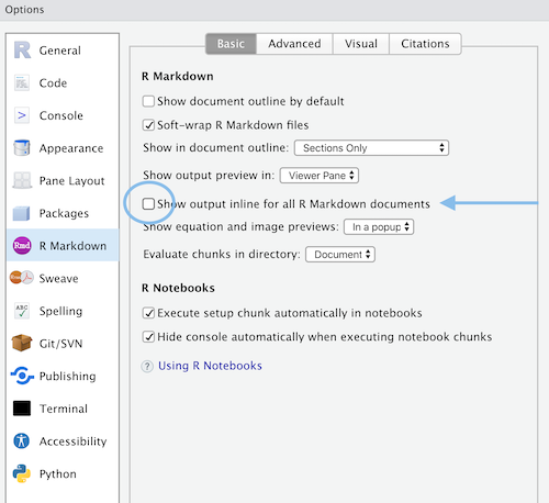
In RStudio, you can remove the inline preview for a code cell. So, instead of the output appearing right below a code cell, the output will appear in the Viewer pane.
This can be done as a global setting in RStudio by going to Tools > Global Options > R Markdown. On that options page, un-check the box that says Show output inline for all R Markdown documents. Don’t worry if you’re using Quarto, this setting applies for those such as well.
Hit the “Apply” button for this setting to take effect.
Your workspace in RStudio should then look something like this:
In this section, we showed you how to develop Quarto documents in RStudio, one code cell at a time. A .qmd file can be used to both save and execute code, and to create a reproducible record of what you did and how you did it.
Rendering
Quarto is designed to keep your source code separate from your output. Why? Because you will want to save your source code as a readable record of what you did. The source code can then be used to “play back” that record and (re-)produce the output. To be reproducible though, you have to first produce something—let’s render this .qmd to produce an output file.
Knitting the source file
1 + 1
The file extension .qmd makes your file executable, which means that this file can be used to both save and execute code. Here is a code cell:
[1] 2Any output your code produces like tables, plots, or other results can be included when you render your document. This process is called rendering, because you are executing code and putting the output back into the document. There is a special button for it in RStudio that looks like this:  .
.
Keyboard shortcuts
NOTE: You may also use keyboard shortcuts to knit:
-
Ctrl+Shift+Kon Windows -
Cmd+Shift+Kon Mac
The output file
When we render that Early Words .qmd file, Quarto generates a new file that now contains four elements:
Metadata at the top (we see the title)
Narrative text
Code cell (but we only see one…)
Results (a plot!)
The great thing about Quarto is that it can render the same source document to a multiple of different output formats.
The output format
This output file made in the previous example is an HTML document. This is a type of format, which was stored in the document’s metadata block:
---
title: "Early words"
format: html
---
Output formats are one of the most versatile features of Quarto—you can use them to build web pages like the one shown above. Going further, you can create Word documents, PDFs, multi-page websites, slides, and even write books.

While this example output is a polished and shareable document as is, it’s not likely that your work stops there—but it is a great place to start. Next, we’ll show how to use Quarto to develop your ideas alongside your code using narrative text.
Writing
Narrative text
Everything that is not code in your .qmd is called narrative text, and can be styled with Markdown. Markdown is a plain text formatting syntax, which means everything you see in the file itself can be typed with a normal keyboard.
Adding structure
You can use Markdown to organize your .qmd file with headings. Headings are useful for organizing your document into sections, and with Markdown formatting you can have up to 6 types/sizes of headers. Use a hash symbol like # before the label to create a new header.
Adding formatting
All narrative text in your .qmd file can be formatted to add bold, italics, bulletted lists, numbered lists, superscripts1, and subscripts1.
How it works
Thus far, we’ve shown how you can use Quarto with RStudio to interactively develop code inside an .qmd document. Next, we showed how you can also take the same .qmd document and knit it to make a single output file, like a simple HTML page. So, you have learned how to fill up an .qmd file with your good ideas, code, and data. How does it all actually work?
The knitr package
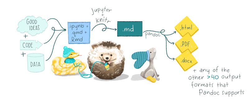
When you click the Render button, Quarto detects your first code cell using the R engine, then feeds the .qmd file to an R package called knitr (https://yihui.org/knitr/) as the code execution engine.
The knitr package executes all of the code cells. Quarto creates a new markdown (.md) document, which then includes your good ideas plus your code and its knitr-generated output (figures, results, tables, etc.).
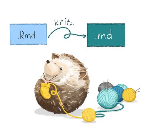
So, knitr turns your .qmd into an .md. This file is no longer executable, but it is still a plain text document without any formatting. Because of this, the actual .md file is temporary and not kept by default.
If you want to keep a copy of the Markdown file after rendering, you can do so using the keep-md option:
---
format: html
execute:
  keep-md: true
---
This is documented on the Quarto website (https://quarto.org/docs/computations/execution-options.html#intermediates).
Pandoc
The markdown file generated by knitr is then processed by a tool called Pandoc (https://pandoc.org/).
Pandoc is a free and open-source document converter. Quarto calls Pandoc for you to create the finished output file. Pandoc also transforms your Markdown-flavored text into formatted text in your final file format.
If you choose a format in your YAML, this is passed to Pandoc to convert the .md into the right format. This is the formatted document that you’ll want to read and share with others.
Rendering from the command line
This may all sound complicated, but Quarto and RStudio makes this simpler for you by wrapping it all up with the “Render” button.
If you don’t use RStudio, or if you simply prefer using the command line, you can also render a .qmd file from the R console using the quarto package.
The quarto_render() function will pass your .qmd file through the same process described above with knitr and Pandoc.
One of the most powerful features of the knitr package is how it helps you control how your code and output look in your final finished product. Want to hide some gnarly-looking code that nevertheless makes a beautiful plot? Want to save all the plots you made in a directory when you knit? Read on to learn about knitr code cell options for figures.
Code Cells
We just learned about how the knitr package is responsible for both executing code and knitting the output back into the document. The knitr package has some special code cell options to control how your code both works and looks.
Using code cell options
All knitr options are placed between the curly braces {} on the first line of each code cell. This line is called the header, and it must be a single line without line breaks.
The option name goes on the left, with the value on the right. You may include spaces around the equal sign if you wish.
```{r echo=FALSE}
...code goes here...
```
Multiple options can be separated by commas. You may include or exclude extra spaces around the comma, too.
```{r echo=FALSE, error=TRUE}
...code goes here...
```
Careful! The r part is the code engine. While other engines are possible, when you edit the header, be sure not to touch the code engine.
In total, there are 56 options, so we’ll highlight those with the highest payoff. Options specific to controlling figures are covered in the next section.
Controlling what appears in the output
By default, all source code, output, warnings, and messages are printed faithfully by knitr in the output file. The most important knitr options help you gain control over what appears in your output when you knit. By combining options, you can have the output display just the code, just the results, both, or neither. For example:
-
echo = FALSEhides code (but not results) from appearing in the output file. This is a useful way to embed figures. -
results = FALSEhides text results from appearing in the output file (the corollary option for figures isfig.show = 'hide') -
message = FALSEhides messages generated by the code cell from appearing in the output file. -
warning = FALSEhides warnings generated by the code cell from appearing in the output file. -
include = FALSEhides code, results, warnings, and messages from appearing in the output file. The code within the code cell is still executed invisibly, and the results can be used by other code cells.
Each of these options takes TRUE or FALSE (no quotes) as its input value, with TRUE as the default value.
Controlling how code is executed
Two additional code cell options help you control how your code is executed when you knit. Note that these do not affect how your code cell run interactively in RStudio.
-
error = TRUEallows the knitting process to keep going if the code cell produces an error. -
eval = FALSEskips executing code in a code cell, often used for code cells where the code calls functions likeinstall.packages()orView(), which should not be run when you knit.
If you find yourself with an .qmd where you want to set error=TRUE or eval=FALSE for all remaining code code cells, you may want to insert code cells strategically using knit_exit(). After that code cell, knitr will exit the knitting process, and all subsequent code cells will be ignored.
```{r include=FALSE}
knitr::knit_exit()
```

The rest of this document is not rendered.
Controlling your entire document
It can get repetitive to reset options for many individual code cells, when sometimes you’d like to override the default values for a whole .qmd document. To set global options that apply to every code cell in a .qmd, call knitr::opts_chunk$set in a code cell.
The setup code cell affects all code cells in the same .qmd document. It is called a global option for that reason.
The option for the setup code cell itself is typically include=FALSE so that no one sees it but you.
```{r setup, include = FALSE}
knitr::opts_chunk$set(
  comment = "#>",
  collapse = TRUE,
  echo = FALSE,
  warning = FALSE,
  message = FALSE
)
```
Knitr will treat each option that you pass to knitr::opts_chunk$set as a global default that can be overwritten in individual headers. You can (and should) use individual options too, but setting up some nice ones that apply to all code cells can save you time and can lessen your cognitive load as you develop your code.
A few notes on what the above options do:
comment = "#>"sets the character on the far left of all printed output such that a reader could copy/paste a block of code into their console and run it (that is, the pasted code with printed output will not produce errors).collapse = TRUEfuses your code cell’s code and output together into a single block (by default, they are written to separate blocks).
Figures
Any figure that you create with code in your .qmd document will be inserted inline into your knitted output file. Previously, we learned about how the knitr package is responsible for both executing code and knitting the output back into the document. When a code cell produces a figure, knitr has some special options available for controlling how your figure looks.
The author makes the graph, saves it as a file, and then copy and pastes it into the final report. This process relies on manual labor. If the data changes, the author must repeat the entire process to update the graph.
Figure placement
By default, plots show up immediately after the code that prints them. For example, the following line plot created with the ggplot package will be inserted when you knit.
ggplot(words, aes(x = age, y = produces, color = lemma)) +
  geom_smooth(se = FALSE, lwd = .5) +
  geom_point(size = 2)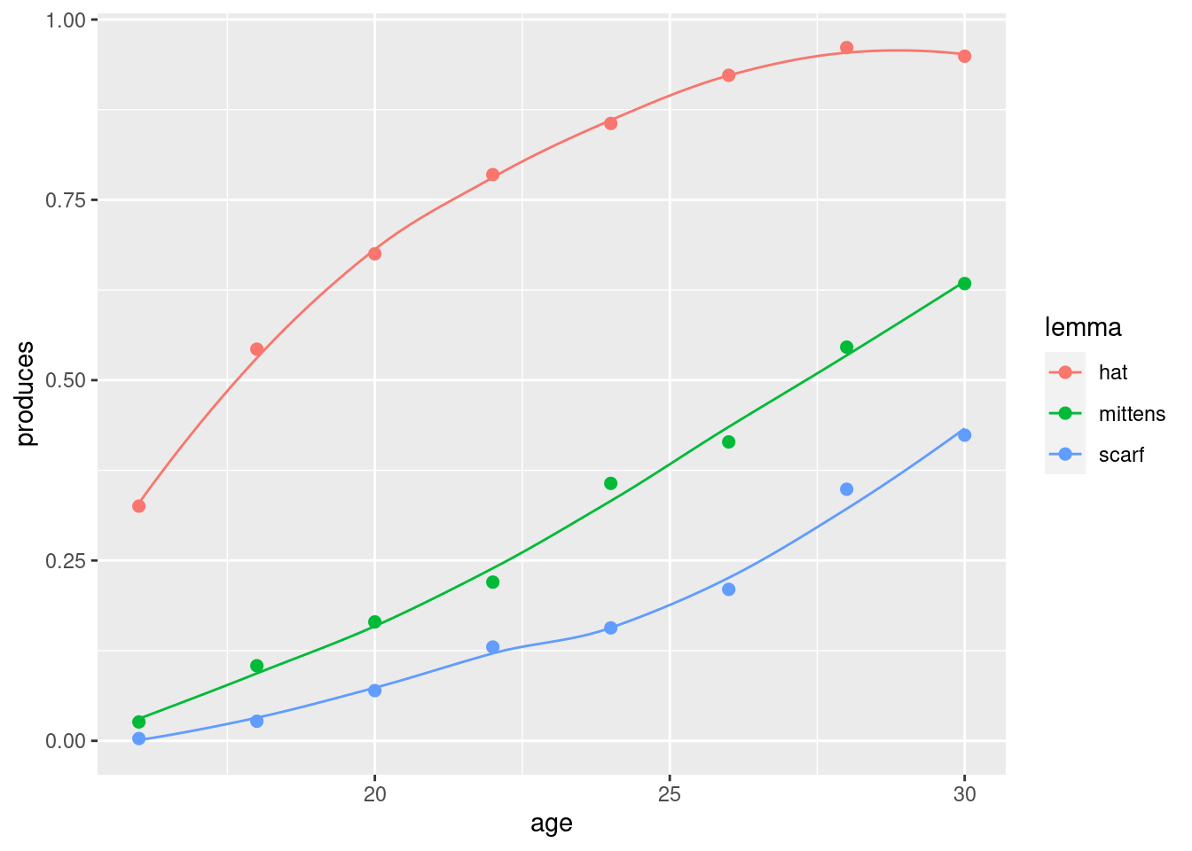
By contrast, the code cell on the below will create a plot object named line. If you ran this code in your console, it would not print the plot until you call the line object by name. The same will be true when you knit.
line <-
  ggplot(words, aes(x = age, y = produces, color = lemma)) +
  geom_smooth(se = FALSE, lwd = .5) +
  geom_point(size = 2)
line
There are two really handy display options for figures:
fig.align = 'center' / 'left' / 'right'aligns the figure in the outputfig.show = 'hide' / 'hold'hides plots entirely, or holds printing until the end of a code cell
You never know when you’ll never options like this but when you’re ready for them, they’re there!
Figure sizing
It can often be hard to get your figures to show up in the right size and place in your knitted output. Some code cell options that help with this are:
out.width = '50%'allows you resize a plot (here, shrunk to half its original size; for full width, set to'100%')fig.asp = 0.618to control the ratio of height to width (this is the golden ratio, but any number will do: < 1 will be more wide than tall)