a_number <- 5
a_number
[1] 5This MVP covers
filter() function, with expressions that filter a table to only the rows you needarrange() function performing several column-selection operations with dplyr’s select() functionmutate() and carefully crafted expressionsgroup_by() and summarize()
We will start off by getting our bearings with assignment of variables in R. Later, we’ll certainly get the opportunity to learn more programming fundamentals, however assignment is one of those topics that should be addressed right away. Then, the installation of packages will be covered. This will give us the chance to install some of required packages: tidyverse, dspatterns, and devtools.
The rest of the section is devoted to learning a skill that is very important: transforming tabular data. Of all the skills you will learn, the value of this one cannot be understated. A bit more than the usual amount of time will and should be spent on this.
The dspatterns package will give us the dataset needed for the examples in this section: sw. This dataset is a modified version of the starwars dataset that is available in the dplyr package. Whenever we load in the dspatterns package using library(dspatterns), the sw table will be available for use. This particular dataset has 87 rows, one for each Star Wars character, and the following 8 variables (or columns):
name: the name of the characterheight, mass: the character’s height and weight (in centimeters and kilograms)hair_color: a description of the character’s hair color, where availablegender, homeworld, species: the character’s gender, homeworld (i.e., a planet name), and speciesWe will learn how to install packages like tidyverse, dspatterns, and devtools. Once you’ve gotten the hang of that (and those packages are installed), more information on the sw dataset can be obtained by executing ?sw in the RStudio console (a help page will appear).
Before we get to the fun stuff, it’s best if we first get acquainted with two things: (1) the programming concept of assignment, and (2) installing packages. We will have a more in-depth look at R programming in later sections and just touch upon the basics for now. In R, installing and using packages is commonplace and thus a fundamental skill, so a few packages will be installed in this section.
Let’s create a new R script using the New File icon in the RStudio toolbar. Now we can type lines of code in the open R Script document in the Source pane, and, also execute individual statements or regions of code by selecting them (as you would select text in a word processor) and using the Control + Enter shortcut.
We assign values to variables (that we name ourselves) by using the leftward arrow <-. Many different types of data can be assigned to a variable. They can be single values, a vector of values (within the c() function, which combines individual values of the same type), or, more complex objects like tables (we’ll get to that in the next section). Let’s have a look at three examples.
We can assign the single number 5 to the variable called a_number. Executing the line with just the variable name prints the value 5 in the console (the assignment line itself will show nothing in the console).
Assigning a single number to a_number.
5 to the variable called a_number.a_number by itself returns the values held by the variable. a_number <- 5
a_number[1] 5Just below the code listing, the console output is shown ([1] 5 in this case).
Multiple values (of the same type, like numbers or character strings) can be put together (with the c() function) as a vector and assigned to a single variable. An example of this is shown in the following code listing.
Assigning a vector of three numbers to three_numbers.
c(), to combine). The name three_numbers is just a name that was made up; it could easily have been called foo. three_numbers <- c(1, 2, 3)
three_numbers[1] 1 2 3Shown again, just above, is the console output. We are getting back the values we put into three_numbers.
Character strings can be assigned to variables. In the next example, the single string "hello" is assigned to one_word.
Assigning a character string to one_word.
one_word <- "hello"
one_word
[1] "hello"The console output shown above consists of all values in one_word: #> [1] "hello".
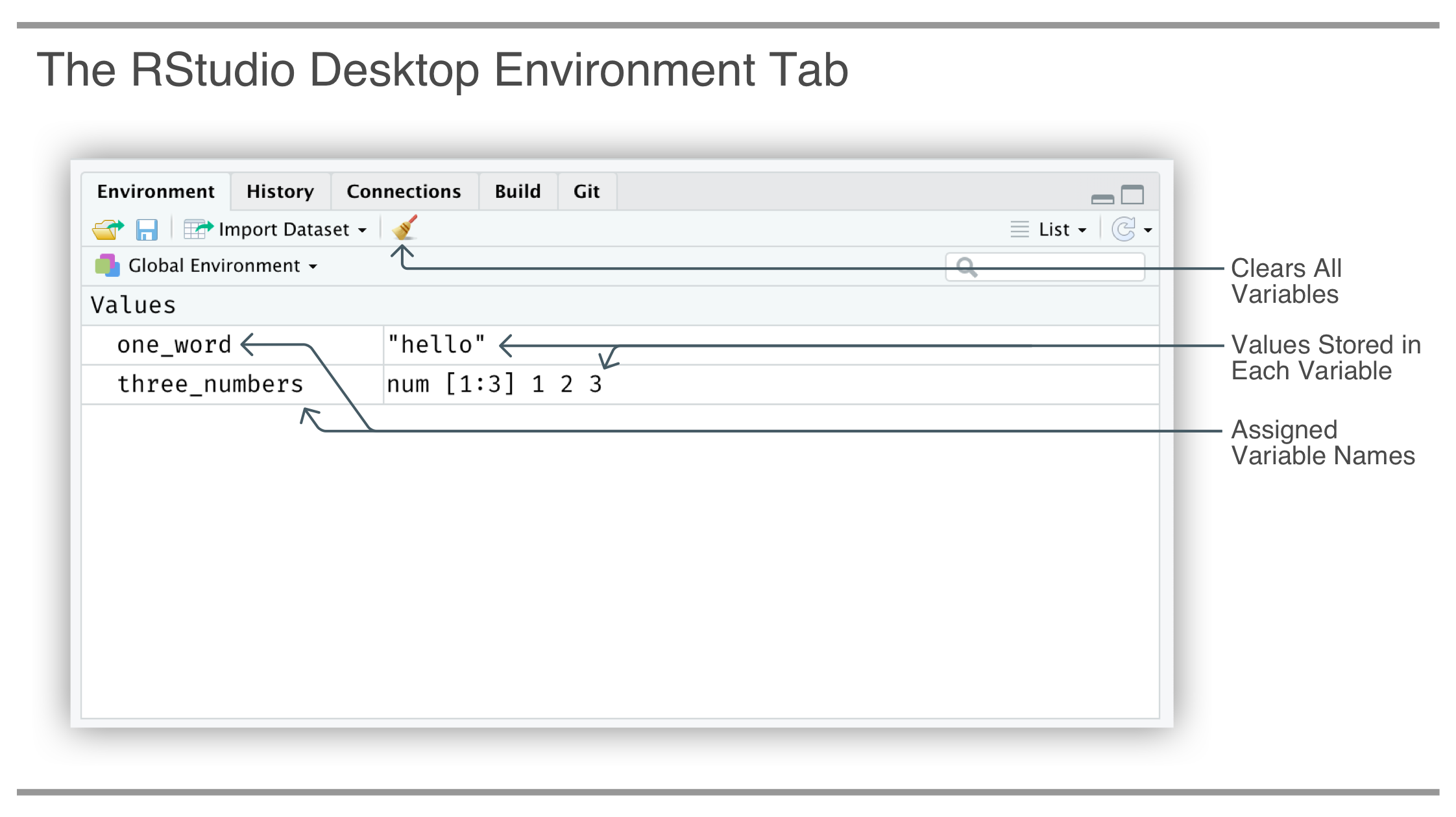
A good way to check that the variables were actually defined is to look at the Environment tab in the top-right pane of RStudio. The names of the variables will appear here as they are assigned, and, you also get an indication of the value attached to the variable.
We can overwrite any variable currently assigned. This is done by assigning a value to any variable name that was previously assigned. In the next example, we’ll overwrite the one_word variable with "hi" and inspect the variable by printing it.
Replacing the one_word variable with a different value.
one_word, and, R won't inform you that one_word was previously assigned. one_word <- "hi"
one_word[1] "hi"The return value in the console is now "hi", or, #> [1] "hi". The Environment tab in RStudio will show us this change after executing the first statement in the previous code listing. The execution, or printing, of just the variable one_word further confirms this in the console.
While visualizing your data is useful for generating insights, it’s not common that you’ll initially have the data in exactly the form you need. It’s far more likely that you first will have to create some new variables or generate some summaries before plotting the data. So, we’ll get to visualization in the next section and learn all transforming our data first. The process of data transformation is made easier in R by using the dplyr package. We’ll learn how to use only a few functions from dplyr to modify a dataset in several useful ways.
There are five key dplyr functions that can help us solve the vast majority of data manipulation tasks:
filter() — Pick observations by their valuesarrange() — Reorder the rowsselect() — Pick variables by their namesmutate() — Create new variables with functions of existing variablessummarize() — Collapse many rows down to a single summaryThese can be used in conjunction with the group_by() function, which tells dplyr that it should be operating on data group-by-group (i.e., with collections of rows). Taken together, these functions enable a cohesive language of data manipulation.
All these functions generally work the same, where
Eventually we’ll see that we can chain together multiple simple steps to achieve a complex result but, first, let’s just see how each of these functions work in isolation.
Through the rest of this section, let’s work with dplyr in the context of an R Markdown document. In the following code listing, we’ll create a new R Markdown document and include this R code chunk just after the YAML header.
Loading the tidyverse and dspatterns packages.
The following is the console output which, in an R Markdown document, appears just below the code chunk (as chunk output).
#> ── Attaching packages ──────────────────────────── tidyverse 1.2.1 ──
#> ✔ ggplot2 3.0.0     ✔ purrr   0.2.5
#> ✔ tibble  1.4.2     ✔ dplyr   0.7.6
#> ✔ tidyr   0.8.1     ✔ stringr 1.3.1
#> ✔ readr   1.1.1     ✔ forcats 0.3.0
#> package 'dplyr' was built under R version 3.5.1── Conflicts
#> ───────────────────────────────────── tidyverse_conflicts() ──
#> ✖ dplyr::filter() masks stats::filter()
#> ✖ dplyr::lag()    masks stats::lag()
After running the chunk (using Shift + Control + Enter or the Run Current Chunk button), you might see messages relating to conflicts: this is entirely normal and expected (so don’t worry about it). Now these packages are loaded, and all of their functions are available to use.
We’ll continue the practice of writing new R code chunks and running them interactively in an R Markdown document. The Environment pane in RStudio will fill up with variables and objects during this progression. Whenever in doubt about whether a variable has or hasn’t been assigned during this sort of ad-hoc data analysis, it is recommended to use the RStudio menu option Session >> Restart R and Clear Output. This provides a clean slate where you can then run the chunks from top to bottom.
sw Dataset and the Elements of a TableThe dataset with the name sw is provided by the dspatterns package. That is, once dspatterns is loaded in the session with library(dspatterns), the sw dataset will be available. R considers datasets to be important components of packages since they are valuable for testing out a package’s functions. It may seem odd, but we can treat sw like a variable that doesn’t have to be explicitly assigned by the user. In the following code listing, we see that just by entering sw in the console, its output is provided.
The sw dataset can be printed to the console by using sw.
library(dspatterns)), we have access to the sw dataset. Executing sw (a tibble) prints it and shows us some of its values. sw# A tibble: 87 × 8
name height mass hair_color birth_year gender homeworld species
<chr> <int> <dbl> <chr> <dbl> <chr> <chr> <chr>
1 Luke Skywalker 172 77 blond 19 mascu… Tatooine Human
2 C-3PO 167 75 <NA> 112 mascu… Tatooine Droid
3 R2-D2 96 32 <NA> 33 mascu… Naboo Droid
4 Darth Vader 202 136 none 41.9 mascu… Tatooine Human
5 Leia Organa 150 49 brown 19 femin… Alderaan Human
6 Owen Lars 178 120 brown, gr… 52 mascu… Tatooine Human
7 Beru Whitesun la… 165 75 brown 47 femin… Tatooine Human
8 R5-D4 97 32 <NA> NA mascu… Tatooine Droid
9 Biggs Darklighter 183 84 black 24 mascu… Tatooine Human
10 Obi-Wan Kenobi 182 77 auburn, w… 57 mascu… Stewjon Human
# ℹ 77 more rowsThe sw dataset is a tibble object, a special implementation of a data frame (a tibble prints its data differently, filling the entire width of the console). We’ll learn a bit more about tibbles in a later section, especially in how else they differ from data frames. For sw, there are more rows in the data than what is shown (we see 6 rows, but there are 81 more that aren’t displayed).
The returned console output for sw has a lot of information. This is a good opportunity to take some time to understand this type of output. The very first line describes the type of object returned, which is a tibble, and it also provides the dimensions of the table (87 rows and 8 columns, or, variables). The second line shows the table’s column names, and the line below that describes each column’s type:
<chr> is for character (or text) data<int> is for integer (numbers without decimal places),<dbl> is for double-precision values which are numeric, except they have a decimal component unlike integersDepending on the width of your editing pane, the printing of the tibble might show more or less of the table data. Columns that don’t fit in the print area are mentioned at the bottom (e.g., ... with 3 more variables: ...) and, with smaller widths of the console or R Markdown editing pane, data in some columns will be more truncated (e.g., showing Obi-Wan Ken... instead of the full name of Obi-Wan Kenobi). While this is intentional, we may want to inspect just a little bit more of the data values. One quick fix is to manually widen the output area (by dragging the center, vertical pane in RStudio left or right) and print the output again. The extra width will provide more space for the individual columns and the output may even show you data in more columns.
Sometimes, you’ll discover a dataset in a package, look at it, and have no context for what the columns are supposed to be indicating. Datasets in R usually have internal help documents that explain the dataset in some detail. Try typing in help(sw) or ?sw in the console, the help document will appear in the Help section in the bottom-right pane in RStudio.
You may have noticed a few of the values in the printed dataset show as NA. Those indicate missing values, perhaps where no observation exists for a particular variable in a row. We can have NA values for all different types of columns (e.g., character, numeric, etc.).
The filter() function allows you to generate a subset of rows with a filtering expression. Let’s filter the sw dataset in the same R Markdown document that we started earlier and get back only those rows where the species is "Droid". The expression to use is species == "Droid". The first argument is the name of the data to transform: sw.
The filter() function, and filtering by a single value in the species column of the sw dataset.
filter() is the data, which is sw; the filtering expression comes next. filter(sw, species == "Droid")# A tibble: 6 × 8
name height mass hair_color birth_year gender homeworld species
<chr> <int> <dbl> <chr> <dbl> <chr> <chr> <chr>
1 C-3PO 167 75 <NA> 112 masculine Tatooine Droid
2 R2-D2 96 32 <NA> 33 masculine Naboo Droid
3 R5-D4 97 32 <NA> NA masculine Tatooine Droid
4 IG-88 200 140 none 15 masculine <NA> Droid
5 R4-P17 96 NA none NA feminine <NA> Droid
6 BB8 NA NA none NA masculine <NA> Droid The table prints out after this transformation (because it wasn’t assigned to a variable). We see from the output that returned table seems to have just those species that are of the "Droid" type.
Filtering expressions are often performed by using comparison operators. The main ones are:
== (equal),!= (not equal),>, >= (greater than and greater than or equal to),<, <= (less than and less than or equal to),%in% (part of a set)Let’s look at an example using a greater than (>) comparison operator. To get a filtered table with all characters with a height more than 220 centimeters, we need to use height > 220.
Filtering to only keep rows where the height column has values greater than 220.
filter(sw, height > 220)# A tibble: 5 × 8
name height mass hair_color birth_year gender homeworld species
<chr> <int> <dbl> <chr> <dbl> <chr> <chr> <chr>
1 Chewbacca 228 112 brown 200 masculine Kashyyyk Wookiee
2 Roos Tarpals 224 82 none NA masculine Naboo Gungan
3 Yarael Poof 264 NA none NA masculine Quermia Quermian
4 Lama Su 229 88 none NA masculine Kamino Kaminoan
5 Tarfful 234 136 brown NA masculine Kashyyyk Wookiee Just by scanning the height column we can see that all values are greater than 220.
There are also logical operators and they can be used to link together filtering statements. These operators consist of the following set:
& (the AND operator)| (the OR operator)The following code filters all Star Wars characters in the sw table to those that either have height above 210 or a mass above 120.
Filtering characters by either height above 210, or, mass above 120.
filter(sw, height > 210 | mass > 120)# A tibble: 10 × 8
name height mass hair_color birth_year gender homeworld species
<chr> <int> <dbl> <chr> <dbl> <chr> <chr> <chr>
1 Darth Vader 202 136 none 41.9 mascu… Tatooine Human
2 Chewbacca 228 112 brown 200 mascu… Kashyyyk Wookiee
3 Jabba Desilijic … 175 1358 <NA> 600 mascu… Nal Hutta Hutt
4 IG-88 200 140 none 15 mascu… <NA> Droid
5 Roos Tarpals 224 82 none NA mascu… Naboo Gungan
6 Yarael Poof 264 NA none NA mascu… Quermia Quermi…
7 Lama Su 229 88 none NA mascu… Kamino Kamino…
8 Taun We 213 NA none NA femin… Kamino Kamino…
9 Grievous 216 159 none NA mascu… Kalee Kaleesh
10 Tarfful 234 136 brown NA mascu… Kashyyyk WookieeWe get back 10 rows (out of 87) with the filtering expression used here. Note that NA values in the mass column are preserved. These rows are present because even though mass is clearly not greater than 120 (it’s missing!), height is still greater than 210.
The next code listing provides another common filtering scenario, where we get just the "Droid" and "Human" species. This subset table can be gotten with at least two different filter() statements. Here is an example that uses two expressions with an OR (|) operator.
Get all Droid and Human characters (method 1 with a [expr | expr] construction).
|), which can be confusing until you think of it in terms of 'include either this or that'. filter(sw, species == "Droid" | species == "Human")# A tibble: 41 × 8
name height mass hair_color birth_year gender homeworld species
<chr> <int> <dbl> <chr> <dbl> <chr> <chr> <chr>
1 Luke Skywalker 172 77 blond 19 mascu… Tatooine Human
2 C-3PO 167 75 <NA> 112 mascu… Tatooine Droid
3 R2-D2 96 32 <NA> 33 mascu… Naboo Droid
4 Darth Vader 202 136 none 41.9 mascu… Tatooine Human
5 Leia Organa 150 49 brown 19 femin… Alderaan Human
6 Owen Lars 178 120 brown, gr… 52 mascu… Tatooine Human
7 Beru Whitesun la… 165 75 brown 47 femin… Tatooine Human
8 R5-D4 97 32 <NA> NA mascu… Tatooine Droid
9 Biggs Darklighter 183 84 black 24 mascu… Tatooine Human
10 Obi-Wan Kenobi 182 77 auburn, w… 57 mascu… Stewjon Human
# ℹ 31 more rowsThe tibble that’s printed shows that, at least in the first 6 rows, each character is either a Human or a Droid.
Next, we provide the better way to get the same result, which is to look for occurrences in a set (defined with the help of c()). So, instead of using species twice in our statement, we can use the %in% operator in a single expression.
Get all Droid and Human characters (method 2 with [colname |> c(...)] construction).
# A tibble: 41 × 8
   name              height  mass hair_color birth_year gender homeworld species
   <chr>              <int> <dbl> <chr>           <dbl> <chr>  <chr>     <chr>
 1 Luke Skywalker       172    77 blond            19   mascu… Tatooine  Human
 2 C-3PO                167    75 <NA>            112   mascu… Tatooine  Droid
 3 R2-D2                 96    32 <NA>             33   mascu… Naboo     Droid
 4 Darth Vader          202   136 none             41.9 mascu… Tatooine  Human
 5 Leia Organa          150    49 brown            19   femin… Alderaan  Human
 6 Owen Lars            178   120 brown, gr…       52   mascu… Tatooine  Human
 7 Beru Whitesun la…    165    75 brown            47   femin… Tatooine  Human
 8 R5-D4                 97    32 <NA>             NA   mascu… Tatooine  Droid
 9 Biggs Darklighter    183    84 black            24   mascu… Tatooine  Human
10 Obi-Wan Kenobi       182    77 auburn, w…       57   mascu… Stewjon   Human
# ℹ 31 more rowsWe get the same output as before. The %in% operator checks for membership in a set (here, "Droid" and "Human" in the species column). This use of %in% is preferred over multiple | operators because there’s less redundancy, it’s much more readable, and it is less error prone to write.
Sometimes, you’ll want to sort your data. The arrange() function makes this possible and it works just like filter() except that instead of selecting rows, it changes their order. It takes the table and a set of column names to order by. If more than one column name is given, each additional column will be used to break ties (if there are still remaining ties, then the original ordering is preserved). Let’s arrange the sw dataset by the height of its characters.
Arranging characters by increasing height.
filter() function (and really, this applies to all of dplyr's main functions), the first value to give to arrange() is the data: sw. arrange(sw, height)# A tibble: 87 × 8
name height mass hair_color birth_year gender homeworld species
<chr> <int> <dbl> <chr> <dbl> <chr> <chr> <chr>
1 Yoda 66 17 white 896 mascu… <NA> Yoda's…
2 Ratts Tyerell 79 15 none NA mascu… Aleen Mi… Aleena
3 Wicket Systri Wa… 88 20 brown 8 mascu… Endor Ewok
4 Dud Bolt 94 45 none NA mascu… Vulpter Vulpte…
5 R2-D2 96 32 <NA> 33 mascu… Naboo Droid
6 R4-P17 96 NA none NA femin… <NA> Droid
7 R5-D4 97 32 <NA> NA mascu… Tatooine Droid
8 Sebulba 112 40 none NA mascu… Malastare Dug
9 Gasgano 122 NA none NA mascu… Troiken Xexto
10 Watto 137 NA black NA mascu… Toydaria Toydar…
# ℹ 77 more rowsWe can see from this snippet of data (6 of 77 rows) that height is increasing (ascending) from top to bottom.
Arranging rows by multiple columns can be a common task and the next example arranges by two different character-based (<chr>) columns: hair_color and then gender.
Arranging characters by hair_color and then by gender.
arrange(sw, hair_color, gender)# A tibble: 87 × 8
name height mass hair_color birth_year gender homeworld species
<chr> <int> <dbl> <chr> <dbl> <chr> <chr> <chr>
1 Mon Mothma 150 NA auburn 48 femin… Chandrila Human
2 Wilhuff Tarkin 180 NA auburn, g… 64 mascu… Eriadu Human
3 Obi-Wan Kenobi 182 77 auburn, w… 57 mascu… Stewjon Human
4 Shmi Skywalker 163 NA black 72 femin… Tatooine Human
5 Luminara Unduli 170 56.2 black 58 femin… Mirial Mirial…
6 Barriss Offee 166 50 black 40 femin… Mirial Mirial…
7 Biggs Darklighter 183 84 black 24 mascu… Tatooine Human
8 Boba Fett 183 78.2 black 31.5 mascu… Kamino Human
9 Lando Calrissian 177 79 black 31 mascu… Socorro Human
10 Watto 137 NA black NA mascu… Toydaria Toydar…
# ℹ 77 more rowsThe sorting is alphabetical and first ordering on hair_color and then ordering on gender for those groups of rows with the same hair_color value. Notice that, in the output, for all the rows where hair_color is "black", the sorting of rows is by "female" first then "male" after that.
We can change the order of any variables to descending with desc(). Let’s modify the previous example so that hair_color is sorted in reverse and gender is still ascending in order.
Arranging by descending hair_color, then by ascending gender.
desc() helper function to indicate that those columns that should be sorted in that way. # A tibble: 87 × 8
name height mass hair_color birth_year gender homeworld species
<chr> <int> <dbl> <chr> <dbl> <chr> <chr> <chr>
1 Jocasta Nu 167 NA white NA feminine Coruscant Human
2 Yoda 66 17 white 896 masculine <NA> Yoda's…
3 Ki-Adi-Mundi 198 82 white 92 masculine Cerea Cerean
4 Dooku 193 80 white 102 masculine Serenno Human
5 Captain Phasma NA NA unknown NA <NA> <NA> <NA>
6 Ayla Secura 178 55 none 48 feminine Ryloth Twi'lek
7 Adi Gallia 184 50 none NA feminine Coruscant Tholot…
8 Taun We 213 NA none NA feminine Kamino Kamino…
9 R4-P17 96 NA none NA feminine <NA> Droid
10 Shaak Ti 178 57 none NA feminine Shili Togruta
# ℹ 77 more rowsWe immediately notice that the first few rows have a hair_color value of "white" (i.e., near the end of the alphabet) and also that gender is indeed sorted in alphabetical order (within the hair_color subgroups).
A final note about the arrange() function: NA values will always be sorted last, and, using desc() doesn’t affect that. Why? Because there is nothing to sort by. NA values are lumped together at the end (although their initial ordering is preserved). And while we are on the topic of NA values, in the above tibble printing, one of the hair_color values should be assigned as an NA value. Which one? The "unknown" one for Captain Phasma. The hair_color values of "none" are perfectly fine as they are because those observations were actually made (of no hair color because, no hair).
It’s not unheard of to be working with datasets having dozens, hundreds, or even thousands of variables. If you’re exploring such a dataset, at some point you’ll likely need to focus on a few variables at a time. The select() function allows us to obtain a useful subset of variables, and, it’s easy to use: provide the names of the variables you want to keep.
Let’s run through a few examples so we can get the general idea. The first example shows how we can get just 3 columns (name, gender, species) from the 8 available.
Selecting the name, gender, and species columns.
select() we first supply the data (sw), and then the columns we want to keep. We separate each name with a comma. select(sw, name, gender, species)# A tibble: 87 × 3
name gender species
<chr> <chr> <chr>
1 Luke Skywalker masculine Human
2 C-3PO masculine Droid
3 R2-D2 masculine Droid
4 Darth Vader masculine Human
5 Leia Organa feminine Human
6 Owen Lars masculine Human
7 Beru Whitesun lars feminine Human
8 R5-D4 masculine Droid
9 Biggs Darklighter masculine Human
10 Obi-Wan Kenobi masculine Human
# ℹ 77 more rowsIndeed, we find columns remain in the transformed table. Also note that the order in which the variables are provided is preserved in the output.
Because the order of variables matters, we can create a slightly different output table with the same columns. In the next code listing we will see that the order of the variables provided will result in same ordering of variables in the output table: gender, species, and then name.
Selecting the gender, species, and names columns (in that order).
gender, species, name. select(sw, gender, species, name)# A tibble: 87 × 3
gender species name
<chr> <chr> <chr>
1 masculine Human Luke Skywalker
2 masculine Droid C-3PO
3 masculine Droid R2-D2
4 masculine Human Darth Vader
5 feminine Human Leia Organa
6 masculine Human Owen Lars
7 feminine Human Beru Whitesun lars
8 masculine Droid R5-D4
9 masculine Human Biggs Darklighter
10 masculine Human Obi-Wan Kenobi
# ℹ 77 more rowsThe output table shows that the order of columns is that which was specified in the select() call.
There are a handful of helper functions you can use within select():
starts_with(): matches column names that begin with certain characters,ends_with(): matches column names that end with specific characters, andcontains(): matches column names that contain a sequence of characters.There aren’t any variables in sw that share a common beginning but there are more than a few with common endings. Let’s get the name column first and then any columns that end with the letter "s".
Selecting the name column and any additional columns ending with "s".
name column (appearing first, at the left) and then all columns with those names ending in the letter "s" (in the order they originally appear). # A tibble: 87 × 3
name mass species
<chr> <dbl> <chr>
1 Luke Skywalker 77 Human
2 C-3PO 75 Droid
3 R2-D2 32 Droid
4 Darth Vader 136 Human
5 Leia Organa 49 Human
6 Owen Lars 120 Human
7 Beru Whitesun lars 75 Human
8 R5-D4 32 Droid
9 Biggs Darklighter 84 Human
10 Obi-Wan Kenobi 77 Human
# ℹ 77 more rowsAs we expect, we get the column called name first then all of the columns ending with "s", in the order that those last two columns appeared in the original dataset.
Noting that there are a few columns in sw that contain the underscore ("_") character, let’s try using the contains() helper function for quickly selecting those column names (along with name).
Selecting the name column and any additional columns containing an underscore.
name column comes first. Any column names containing an underscore character will follow (in their original order). # A tibble: 87 × 3
name hair_color birth_year
<chr> <chr> <dbl>
1 Luke Skywalker blond 19
2 C-3PO <NA> 112
3 R2-D2 <NA> 33
4 Darth Vader none 41.9
5 Leia Organa brown 19
6 Owen Lars brown, grey 52
7 Beru Whitesun lars brown 47
8 R5-D4 <NA> NA
9 Biggs Darklighter black 24
10 Obi-Wan Kenobi auburn, white 57
# ℹ 77 more rowsAside from the name column, we see the columns with underscores populating the rest of the tibble printout.
If ever we want to put a few columns near the start and keep other columns in the same order then the everything() select helper function is useful for this.
Selecting three specific columns and then everything() else after that.
everything()). select(sw, name, homeworld, gender, everything())# A tibble: 87 × 8
name homeworld gender height mass hair_color birth_year species
<chr> <chr> <chr> <int> <dbl> <chr> <dbl> <chr>
1 Luke Skywalker Tatooine mascu… 172 77 blond 19 Human
2 C-3PO Tatooine mascu… 167 75 <NA> 112 Droid
3 R2-D2 Naboo mascu… 96 32 <NA> 33 Droid
4 Darth Vader Tatooine mascu… 202 136 none 41.9 Human
5 Leia Organa Alderaan femin… 150 49 brown 19 Human
6 Owen Lars Tatooine mascu… 178 120 brown, gr… 52 Human
7 Beru Whitesun la… Tatooine femin… 165 75 brown 47 Human
8 R5-D4 Tatooine mascu… 97 32 <NA> NA Droid
9 Biggs Darklighter Tatooine mascu… 183 84 black 24 Human
10 Obi-Wan Kenobi Stewjon mascu… 182 77 auburn, w… 57 Human
# ℹ 77 more rowsHere we notice that we do get the name, homeworld, and gender columns first, and then every other remaining column (in their preserved order):
These select helper functions are very useful. They save us having to carefully type out every column name, which can be arduous and error-prone if we have a very large number of columns.
We can create new columns of data with mutate(). It adds the new variables at the end of the table, so, let’s prepare a narrower version of sw by using select().
Create the sw_small table containing just three columns.
select() three columns from sw and assign the resulting table to sw_small.sw_small) displays that smaller table in the output. sw_small <- select(sw, name, height, mass)
sw_small# A tibble: 87 × 3
name height mass
<chr> <int> <dbl>
1 Luke Skywalker 172 77
2 C-3PO 167 75
3 R2-D2 96 32
4 Darth Vader 202 136
5 Leia Organa 150 49
6 Owen Lars 178 120
7 Beru Whitesun lars 165 75
8 R5-D4 97 32
9 Biggs Darklighter 183 84
10 Obi-Wan Kenobi 182 77
# ℹ 77 more rowsNow, let’s take the new sw_small table and create a new column called bmi and calculate the body mass index for all characters in the next code listing. The mathematical expression uses column names to generate a row-wise calculation result. Here we use the right-hand side (RHS) expression: mass / (height / 100)^2. On the left-hand side (LHS) of the expression is the new column bmi.
Add the bmi column to sw_small using the mutate() function.
mutate() function takes data first (sw_small) and then an expression that creates the new column bmi. The expression uses values from the mass and height columns and places the results in the bmi column. mutate(sw_small, bmi = mass / (height / 100)^2)# A tibble: 87 × 4
name height mass bmi
<chr> <int> <dbl> <dbl>
1 Luke Skywalker 172 77 26.0
2 C-3PO 167 75 26.9
3 R2-D2 96 32 34.7
4 Darth Vader 202 136 33.3
5 Leia Organa 150 49 21.8
6 Owen Lars 178 120 37.9
7 Beru Whitesun lars 165 75 27.5
8 R5-D4 97 32 34.0
9 Biggs Darklighter 183 84 25.1
10 Obi-Wan Kenobi 182 77 23.2
# ℹ 77 more rowsWe can see that the column bmi is now available to the right of the original columns name, height, and mass. All new columns that are created by mutate() are placed at the end (which is to the right). The bmi column has values in every row (this is a double-type variable, since mass is of the type double).
It turns out that the mutate() function is very powerful. We can have multiple mutations in a single call of mutate(). What’s even more interesting (and useful) is that a variable created in an expression is immediately available for use in a following expression (in the same mutate() call).
Add the bmi column as before and then create bmi_rnd.
mutate() statement is a bit longer than the last so let's split it over a few lines.bmi column and its values (just like in the last example).bmi_rnd column, a rounded version of bmi (with no decimal places). # A tibble: 87 × 5
name height mass bmi bmi_rnd
<chr> <int> <dbl> <dbl> <dbl>
1 Luke Skywalker 172 77 26.0 26
2 C-3PO 167 75 26.9 27
3 R2-D2 96 32 34.7 35
4 Darth Vader 202 136 33.3 33
5 Leia Organa 150 49 21.8 22
6 Owen Lars 178 120 37.9 38
7 Beru Whitesun lars 165 75 27.5 28
8 R5-D4 97 32 34.0 34
9 Biggs Darklighter 183 84 25.1 25
10 Obi-Wan Kenobi 182 77 23.2 23
# ℹ 77 more rowsWhile bmi is calculated just as before, there is a second expression to create another column. In that second expression, bmi is used in a rounding statement (rounding to 0 decimal places) to create the bmi_rnd variable.
To get summary statistics across a set of groups we can use group_by() in conjunction with summarize(). The summarize() function works a lot like mutate() in that we can provide a new column name and a statement for its calculation. We can use several different aggregation functions inside summarize(): mean(), median(), sd(), min(), max() are the common ones. The summarize() function is typically used right after the group_by() function, which creates grouped data. Several examples will be useful to show us how this works.
Let’s group by species and get the mean of the mass variable for each group. First, we’ll make grouped data in a separate object and then we can generate a summary of the average mass for each species.
Grouping by the species variable and summarizing to get the mean mass.
sw, and grouping it by the species column. That's assigned to the by_species object.by_species object, now a grouped table, is the data for the summarize() statement. For each of group of species we get a row of the average mass per group. # A tibble: 38 × 2
species avg_mass
<chr> <dbl>
1 Aleena 15
2 Besalisk 102
3 Cerean 82
4 Chagrian NA
5 Clawdite 55
6 Droid NA
7 Dug 40
8 Ewok 20
9 Geonosian 80
10 Gungan NA
# ℹ 28 more rowsNotice that we get two columns back: one is from the species group and one is from the column we defined in the summarize() statement (avg_mass).
The pattern will hold that we get all grouping columns and all summary columns back. Another observation here is that some values for avg_mass appear as NA. This occurs if any NA values are introduced to mean(), the result will invariably be NA (the behavior holds true for the other aggregation functions as well). To circumvent this, we can exclude NA values in the calculation of the mean by using the na.rm = TRUE option within mean(). Let’s now revise that summarize() statement.
A slight modification to the summary expression to deal with missing (NA) values.
mean() expression used inside summarize() some of the NA values are replaced with non-NA (i.e., numeric) values. # A tibble: 38 × 2
species avg_mass
<chr> <dbl>
1 Aleena 15
2 Besalisk 102
3 Cerean 82
4 Chagrian NaN
5 Clawdite 55
6 Droid 69.8
7 Dug 40
8 Ewok 20
9 Geonosian 80
10 Gungan 74
# ℹ 28 more rowsNow we see that all values in the avg_mass column are non-NA, however, there is now at least one NaN (not a number) value. This is explainable. The cause of this stems from there not being any non-NA values for that species. The consequence is that a mean couldn’t be calculated, so R returned an NaN.
Let’s create a summary containing two grouping columns (species and gender) and two summary columns (avg_mass and avg_height) to further demonstrate what can be done with the group_by()/summarize() combination.
Grouping by two columns and obtaining a summary with two new columns.
species and gender; each unique combination is a separate group.summarize() statement will give us four columns: two for the two different groups, and two for the summary columns (avg_mass and avg_height). grouping <- group_by(sw, species, gender)
summarize(
grouping,
avg_mass = mean(mass, na.rm = TRUE),
avg_height = mean(height, na.rm = TRUE)
)# A tibble: 42 × 4
# Groups: species [38]
species gender avg_mass avg_height
<chr> <chr> <dbl> <dbl>
1 Aleena masculine 15 79
2 Besalisk masculine 102 198
3 Cerean masculine 82 198
4 Chagrian masculine NaN 196
5 Clawdite feminine 55 168
6 Droid feminine NaN 96
7 Droid masculine 69.8 140
8 Dug masculine 40 112
9 Ewok masculine 20 88
10 Geonosian masculine 80 183
# ℹ 32 more rowsThis yields four columns as we may have expected. The summarize() function has an interface consistent with mutate(), easily allowing for multiple expressions (separated by commas) where the names we provide on the LHS are the names of the new columns.
|>)Imagine that we want to get a ranking of average BMI values for the human characters across the different home worlds. Using what you know about dplyr, you might write code like this
Bringing it all together with multiple dplyr functions and assigning each step to a different object.
filter() statement, assigning the output table to humans (a sensible, short name).mutate() statement, assigning the output table to humans_bmi (not a bad name).group_by() statement, assigning the output table to humans_avg_bmi_by_homeworld (kind of a long name!).summarize() statement, assigning the output table to humans_avg_bmi_by_homeworld (an even longer name, but it makes sense).arrange() statement, assigning the output table to... an extremely long and redundant name. I'm getting some name fatigue here.humans <- filter(sw, species == "Human")
humans_bmi <-
mutate(
humans,
bmi = mass / (height / 100)^2
)
humans_bmi_by_homeworld <- group_by(humans_bmi, homeworld)
humans_avg_bmi_by_homeworld <-
summarize(
humans_bmi_by_homeworld,
avg_bmi = mean(bmi, na.rm = TRUE)
)
humans_avg_bmi_by_homeworld_sorted <-
arrange(humans_avg_bmi_by_homeworld, desc(avg_bmi))
humans_avg_bmi_by_homeworld_sorted# A tibble: 16 × 2
homeworld avg_bmi
<chr> <dbl>
1 Bestine IV 34.0
2 Tatooine 28.9
3 Bespin 25.8
4 Corellia 25.7
5 Socorro 25.2
6 <NA> 23.9
7 Haruun Kal 23.8
8 Concord Dawn 23.6
9 Kamino 23.4
10 Stewjon 23.2
11 Naboo 22.4
12 Alderaan 22.1
13 Serenno 21.5
14 Chandrila NaN
15 Coruscant NaN
16 Eriadu NaN This output is fine but the code is more than a little frustrating to write because we have to give each intermediate table object a name. We’re just going to use it as input to the next statement, so, we don’t care much about it. As ever, naming things is hard and the process of thinking of meaningful and distinct names will invariably slow down our analysis.
There is another way! It involves using the pipe operator (|>). In the next code listing, we can take a similar set of statements as above and rewrite them in a much more succinct manner (and the final table is exactly the same as before).
Bringing it all together with multiple dplyr functions: this time using the pipe operator.
sw) and pass it into the next function with the pipe (|>).filter() statement is the first transformation step. We don't need to specify the data, filter() already has it thanks to the pipe.mutate(), because we used |> just before.homeworld.summarize().avg_bmi with the arrange() function. The |> operator, the pipe, makes the code easier to both write and read later on. The focus is now on the transformations. A good way to reason about the pipe operator is to think of |> as meaning “then”. Now we can imagine reading the above code as a series of imperative statements: filter, and then mutate, and then group, and then summarize, and then arrange. Let’s rewrite the above statement as pseudocode to make clear that we have a series of imperative statements that can be read in a left-to-right manner:
Using pseudocode to demonstrate the readability of the code in the previous listing.
# Get a table of average BMI values for humans across
# the different worlds in a single, piped expression;
# The following is written as pseudocode
# (don't run it, just read it)
<assigning to bmi_sorted> <-
  <start with the starwars table> %{then}%
  <keep only the rows where species is “Human”> %{then}%
  <create a new column called bmi using a calculation> %{then}%
  <create a group for each unique value in homeworld> %{then}%
  <for each group create a summary table (one col: avg_bmi)> %{then}%
  <order the rows by decreasing avg_bmi value>

<view bmi_sorted>
This pseudocode should roughly map to what we should be thinking when writing out dplyr statements. With a bit of practice, the process of transforming tabular data starts to become natural and the idea of a grammar of data manipulation begins to make more sense.
Your data may not have exactly what you’d like to plot. It’s a reality that’s all too common but we can do something about since we learned the basics of dplyr. We will make some transformations to the dmd table to make a plot we otherwise couldn’t before. Before showing the actual transformation statements, let’s have a look at the plan and rationale for the work.
Suppose we would like to have a new measure that provides the value of a diamond by weight. This is a simple calculation that divides the price of a diamond by its number of carats (price / carats). The new cost per carat variable (cpc) can be easily added to the dmd table by using dplyr’s mutate() function by taking dmd and piping it to mutate(): dmd |> mutate(cpc = price / carats).
Now that we have the cpc variable, taken as a better measure of the worth of a diamond based on its qualities, we can divide the entire set of diamonds into two price classes: those with higher cpc than the median cpc value, and those that are lower. We won’t describe in detail how to get the median cpc value, so we’ll accept that it is around $3,460 per carat. Within our second mutate() statement, we will use ifelse() to get a new price_class variable. The next code listing takes the dmd dataset and applies both mutate() statements to dmd and assigns the result to dmd_mod.
Modifying dmd to obtain two new columns: cpc and price_class.
mutate() statement creates the cpc column...mutate() call makes the price_class column. We haven’t yet used mutate() with ifelse() so let’s examine this more closely. The ifelse() statement used here checks every row of the table for whether cpc is greater than or equal to 3460. For each row where that statement is true, the value in the new price_class column will be given "Above Median". If not true, then the value will be "Below Median".
For our third and final mutate(), we will suppose that diamonds with cut and clarity labeled as The Best should be high-quality diamonds, and thus fetch higher prices. Another ifelse() is to be used within the mutate() statement, creating a new variable called quality. The following listing augments the earlier code with a third mutate().
A third and final mutate() statement to add the quality column to our modified dataset (dmd_mod).
mutate() statement (that creates the quality column) is pretty long so it's broken across a few lines for better readability In the code listing, we are using ifelse() within the third mutate() statement to check for the dual condition of both cut and clarity being equal to "The Best". Those diamonds for which the statement is true will have a quality label that is "Top Drawer". Otherwise, all other diamonds will get a label of "The Rest".
Once we have modified dmd and assigned the results to a new object called dmd_mod, we can make a different type of plot that uses the newly-created variables of price_class and quality. Faceting will be done on the price vs. carats plot, using the new variables in the facet_wrap() statement to create a 2-by-2 plot that compares data points by two quality categories and two price categories.
Modifying dmd to add three new columns, and, plotting dmd_mod with the new variables.
mutate() call.price_class and quality). dmd_mod <-
dmd |>
mutate(cpc = price / carats) |>
mutate(price_class = ifelse(
cpc >= 3460, "Above Median", "Below Median"
)
) |>
mutate(quality = ifelse(
cut == "The Best" & clarity == "The Best",
"Top Drawer", "The Rest"
)
)
ggplot(dmd_mod, aes(x = carats, y = price)) +
geom_point() +
facet_wrap(
facets = vars(price_class, quality),
labeller = label_both
) +
labs(x = "Carats", y = "Price")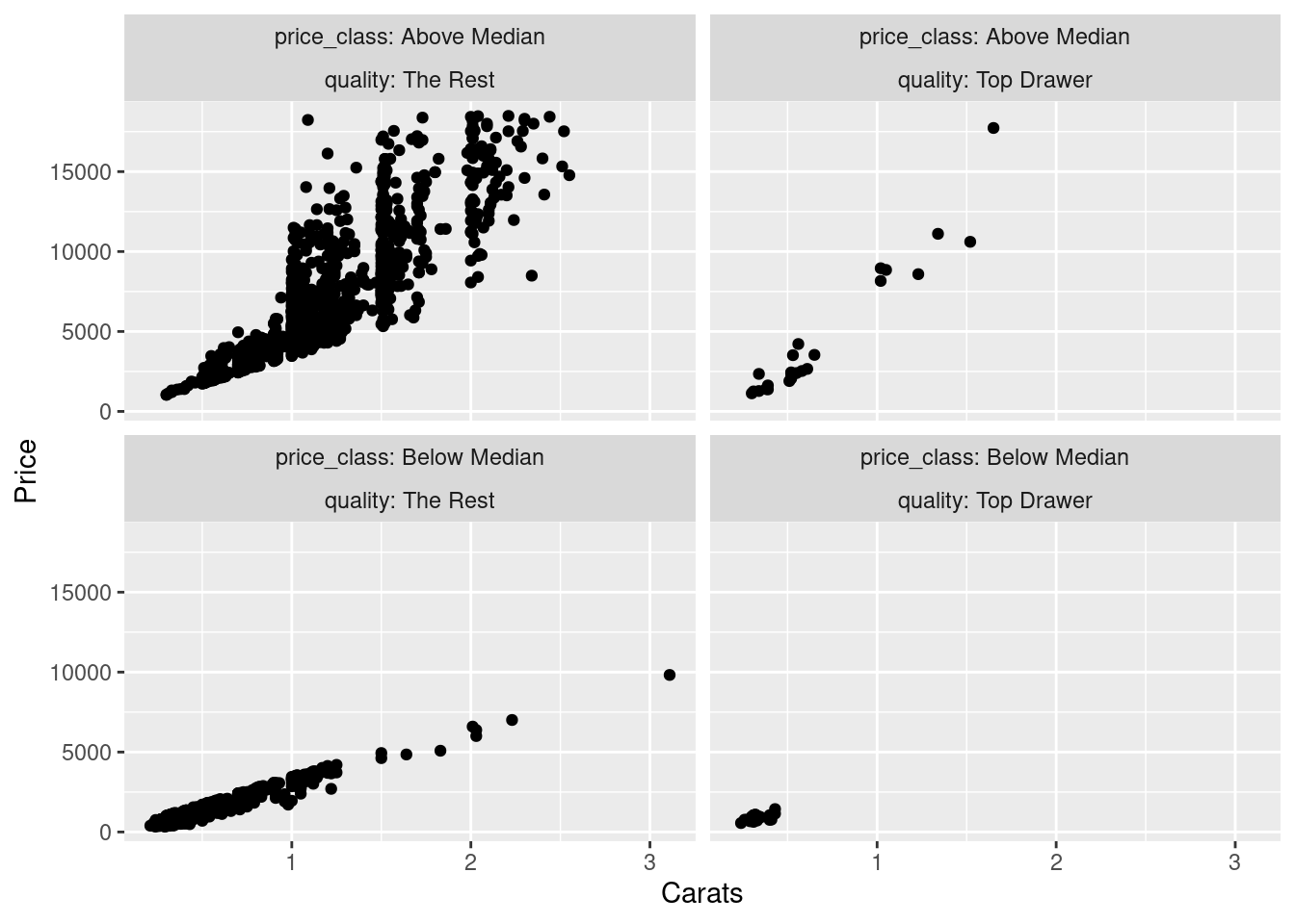
Moving between data transformation activities and plotting with ggplot like this is often valuable for better expressing the data you have to an audience, or, for exploring the data and getting insightful views that were otherwise hidden. Getting to a stage where you can rapidly translate your analysis/visualization needs to raw dplyr & ggplot code is worth the effort and understandably takes some practice.
<- operatorfilter(), arrange(), select(), mutate(), and summarize() (with group_by())|>) (which was used with the dplyr functions) improved the composition and readability of our R statementstibble() and tribble() functions to create our own data tablesWhen you are creating a new R Markdown document for analysis, what set of R statements is likely required before any analysis?
What’s the difference between = and ==? Where should these used (and not used)?
What do you expect to be returned with a filter statement like filter(sw, species == "kangaroo")? There are no kangaroos in Star Wars, so what might happen? (Try it out.)
When the tibble output reads # A tibble: 3 x 8, what do the 3 and 8 correspond to?
What is the difference between these two filter() statements: (1) filter(sw, species == "Human" & mass > 100) and (2) filter(sw, species == "Human" | mass > 100)? Which one would be expected to yield more rows?
You may have noticed that in the statement filter(sw, species %in% c("Droid", "Human")), the word species is not in quotes. Why do you think this is?
When ordering rows with the statement arrange(sw, gender, hair_color), what is the significance of having gender first and hair_color second? What would you expect with a statement like arrange(sw, desc(gender), hair_color)?
Selecting columns is done with select() and select helper functions can be used within that. What selection of columns would occur if you used the statement select(table, name, weight, height, ends_with("t")) on the table with columns name, height, ticket, weight, and city?
How do we drop columns from a table? Say we had a table with the columns name, height, ticket, weight, city and we don’t want the ticket column. How would you write the select() statement?
How do you drop multiple columns from a table? What select() statement could be used on a table with the columns name, height, ticket, weight, and city that would result in leaving in the columns name, height, and weight?
What does the everything() helper function do inside of a select() statement?
Recall that the sw_small table was a narrower version of sw table, with only the name, height, and mass variables. What would result from the statement mutate(sw_small, less_mass = mass - 10)?
Taking once again the sw_small table, do the following two statements result in the same values within the bmi column? Here are the statements: (1) mutate(sw_small, hgt2 = (height / 100)^2, bmi = mass / hgt2), (2) mutate(sw_small, bmi = mass / (height / 100)^2).
Write a mutate() statement with the sw_small table that creates the log_mass variable, which is a calculation of the log of the mass of each character.
What output table would you expect from the statement group_by(sw_small, species)?
What does the summarize() function do?
How many columns are available in the table generated by the statement summarize(group_by(sw, species), avg_mass = mean(mass))?
What’s one helpful thing that the pipe (|>) does?
How would you rewrite the statement in Q17 with the use of the |> operator?
When using the piped statements of sw |> filter(species == "Human") |> mutate(bmi = mass / (height / 100)^2) |> group_by(homeworld), what extra information do you get in the tibble printout?
One or more library() statements should ideally come first to load in package functions. For this lesson, the statements could be library(tidyverse) and library(dspatterns) (to use the datasets and functions suitable for the book content).
The = symbol is an assignment operator, whereas == is a comparison operator. Like the name implies, = is used for assignment (e.g., inside function calls where you’d like to use the argument name and the bound value) and == is used for comparisons (e.g., in expressions that the filter() function uses as a filtering condition).
You get an empty tibble! Dimensions provided are 0 rows by 8 columns. No error: this provides usable output to pass on to other functions.
The 3 corresponds to rows and the 8 represents columns (or variables). It’s customary to represent table dimensions with rows first and then the columns.
The first filter() statement using & will return only those rows describing a "Human" with a mass greater than 100. This is more restrictive than the second filter() statement using |, which returns those rows describing a "Human" or any rows where mass is greater than 100 (not exclusive to Humans). The second statement returns more rows than the first statement.
The word species is not in enclosed in quotes because it represents a column. The dplyr convention is that column names are not surrounded by quotation marks.
The sequence of column names in an arrange() statement directs dplyr to prioritize sorting by the columns provided first. With the statement arrange(sw, desc(gender), hair_color) sorting is still prioritized by gender except that’s a descending sort and the secondary sorting by hair_color is an ascending sort.
The resulting selection of columns would be name, weight, height, and ticket.
Columns are dropped in a select statement by preceding the column name with a hyphen (e.g., select(<table>, -<column_name>)). For the table where we’d want to exclude the ticket column, a suitable statement would be select(<table>, -ticket). Alternatively, we can also write select(<table>, name, height, weight, city), however, this approach becomes less practical when the table has significantly more variables.
Multiple columns can be dropped by prefixing a hyphen to all columns we want to drop. To end up with the columns name, height, and weight from the table with the columns name, height, ticket, weight, and city we can write select(table, -ticket, -city). There is also another way. We can combine the columns we want to exclude in c() and prefix that with a hyphen, as in: select(table, -c(ticket, city)).
The everything() helper function, when inside of a select() statement, provides the remainder of columns that weren’t used explicitly. It can be thought of as “the rest of the columns in the table that I didn’t call out by name”.
The statement mutate(sw_small, less_mass = mass - 10) would add a new variable called less_mass where the value is 10 less than that found in mass (except when mass is NA, whereby less_mass also becomes NA).
The values within the bmi column for both tables will be the same. Notably, with the first statement, we’ll end up with a table that has a hgt_2 column and we probably won’t find that variable very valuable.
The mutate() statement could very well be: mutate(sw_small, log_mass = log(mass)).
With the statement group_by(sw_small, species) you get the same table as sw_small! This is because we just defined some grouping (on species) but we didn’t do anything yet with the groups.
The summarize() function helps us apply one or more aggregation functions (like sum(), mean(), min(), max(), etc.) on grouped data. We get back one summary row per group.
When using the statement summarize(group_by(sw, species), avg_mass = mean(mass)), we get back a summary table with two columns: species (the grouping column) and avg_mass (the column we define in the summarize() function call).
The pipe (|>) is helpful because: (1) it eliminates to need to create intermediate object names for functions that work well with the pipe, and (2) it can be more readable than nested function calls.
The Q17 statement can be rewritten with the pipe as: sw |> group_by(species) |> summarize(avg_mass = mean(mass)).
In the tibble printout, we get information on the groups we made from the group_by() statement. It provides the number of groups and lists the group names alongside that.