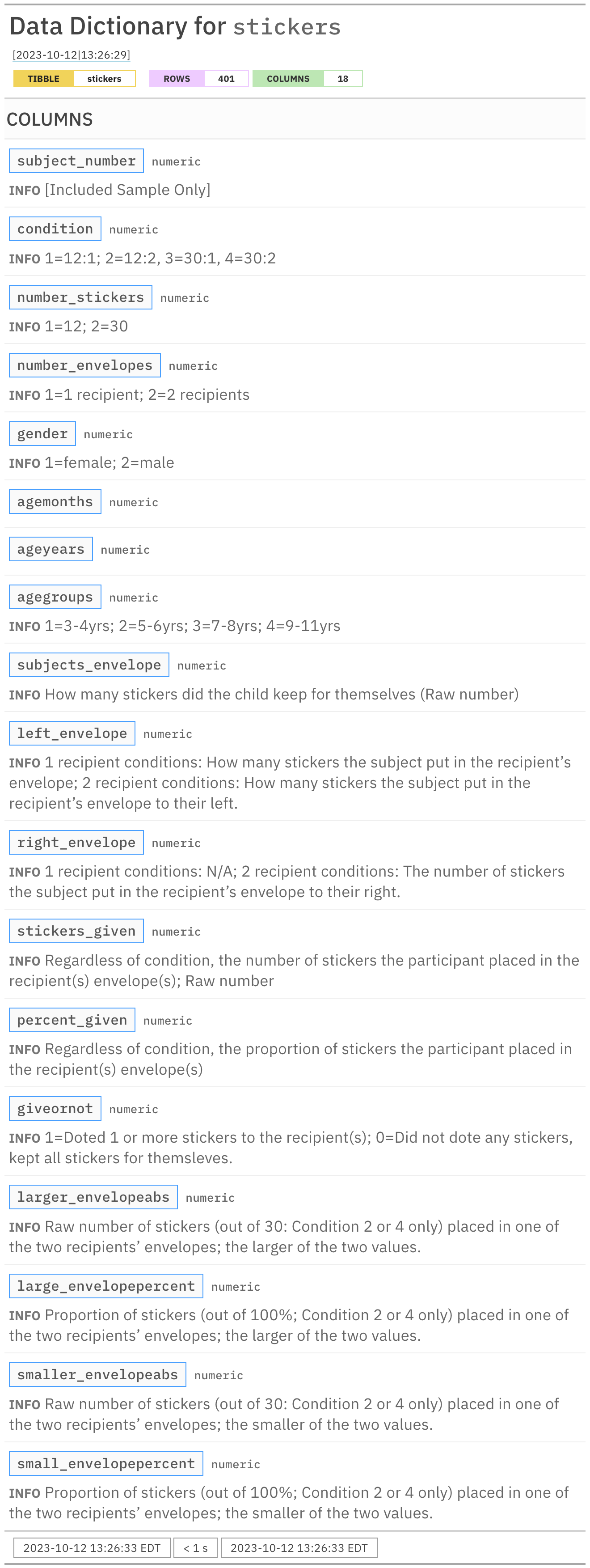
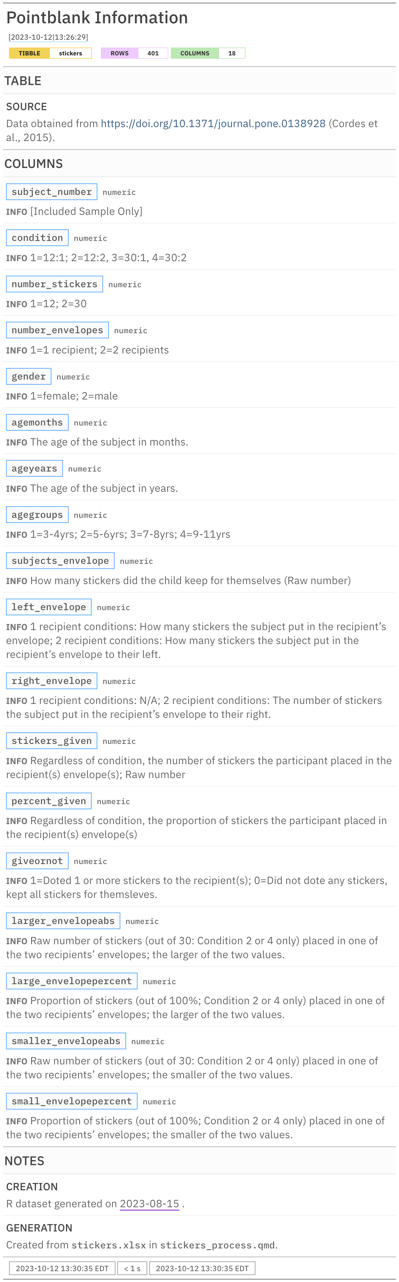
5  Importing Data for the First Time

Explore: The first steps with a new pattern (e.g., get info you need, take stock, smell checks).

Understand: Learning anything can involve asking questions (what kinds? How to actually translate to code? Interpreting outputs personally, may lead to more exploration).

Explain: How do we take the answers and rationalize with the investigations? That’s covered in this pattern. How to document to oneself, programmatic text for resilient reporting. This is really about talking to yourself, in a way.

Share: Communication and collaboration. We’ll show you ways you can make everything presentable and create outputs in a format that allows for easy consumption and feedback. An example: reordering plots or tables to make them easier to interpret.

In this chapter we’ll get down and dirty with some messy data. We need to use this data and although we acknowledge the data has problems, we can use a few strategies to overcome this.

First, we’ll explore the data and find out what went wrong during the import phase. This will invariably require some trial-and-error at first to get to a usable solution (which is the ideal import statement for the dataset at hand). After that, we’ll use functions like glimpse(), count(), head(), and tail() to make sense of what we have during every step of the process. Checking the data at every major transformation is informative and important during this early phase of exploring a new dataset.

All of this work will inevitably result in a messy .qmd file but you’ll leave it in the dust when you’re finally able to diagnose all of the issues. (We recommend you save the file for later use and we’ll provide a tip or two on how to organize these scratch files.)

We’ll need a few packages loaded in for this chapter:

If you’re following along, add a set of library() statements at the top of your .qmd file.

5.1 Explore

Getting new data can be really exciting but it can often result in a lot of work. You have to import the data such that it’s not a garbled mess, you have to understand how the data is organized, and, you may have to do some cleaning and data quality tasks. The first few times you do this can be an exercise in frustration, involving much messing around until you feel you have a handle on things. That said, the goal of this chapter is to provide you with some workflows and many tips/tricks that’ll serve you well when onboarding new datasets.

We’ll be working with an Excel file called stickers.xlsx in this chapter (the file is available in the book repository). The dataset has a lot to do with sharing stickers and it’s a really interesting one. The problem is that the data in its Excel form is a bit problematic (there’s a few problems to overcome).

Putting the problems aside for now, let’s learn about where this dataset came from. It’s a dataset from an experimental study where children played a variation of the dictator or ultimatum game, using stickers instead of money. The study looked at how numerical context affects children’s sharing behavior.

A schematic of the ultimatum game.

The authors made that dataset freely available so we in turn get the chance to examine it in R. Let’s read in the file with the readxl package (with the read_excel() function) and have a first look at the data table.

read_excel("stickers.xlsx")
# A tibble: 402 × 18
   SubjectNumber       Condition NumberStickers NumberEnvelopes Gender Agemonths
   <chr>               <chr>     <chr>          <chr>           <chr>      <dbl>
 1 [Included Sample O… 1=12:1; … 1=12; 2=30     1=1 recipient;… 1=fem…        NA
 2 1                   1         1              1               1             36
 3 2                   1         1              1               2             36
 4 3                   1         1              1               2             36
 5 4                   1         1              1               1             36
 6 5                   1         1              1               2             36
 7 6                   1         1              1               2             36
 8 7                   2         1              2               1             36
 9 8                   2         1              2               2             36
10 9                   3         2              1               2             36
# ℹ 392 more rows
# ℹ 12 more variables: Ageyears <dbl>, Agegroups <chr>,
#   `Subject'sEnvelope` <chr>, LeftEnvelope <chr>, RightEnvelope <chr>,
#   `absolutenumberofstickersgiven(Conditions1or3:Outof12;Conditions2or4:Outof30)` <chr>,
#   `PercentGiven(Outof100percent)` <chr>, Giveornot <chr>,
#   LargerEnvelopeabs <chr>, LargeEnvelopepercent <chr>,
#   SmallerEnvelopeabs <chr>, SmallEnvelopepercent <chr>

Okay, a few things stick out as being non-ideal. First, we seem to have an extra ‘header’ row that got into the table rows (as row 1). It contains notes and remarks about data encoding. We don’t want that, so let’s try using the skip option that’s available in readxl::read_excel(). We need to provide some number of rows and while we can try 1 and 2, they don’t quite work (try using read_excel("stickers.xlsx", skip = 1) and read_excel("stickers.xlsx", skip = 2) and take note of the output table).

Because the rows to skip begin after the row with the column names, we’ll have to try a different strategy. It’ll seem a bit strange but the idea will be to get the column names separately and then all of the good data rows. First, let’s get those column names, and we can do that with n_max = 0 in the read_excel() call:

stickers_empty <- read_excel("stickers.xlsx", n_max = 0)

This gives us a tibble with no rows, but with the column names nonetheless:

stickers_empty
# A tibble: 0 × 18
# ℹ 18 variables: SubjectNumber <lgl>, Condition <lgl>, NumberStickers <lgl>,
#   NumberEnvelopes <lgl>, Gender <lgl>, Agemonths <lgl>, Ageyears <lgl>,
#   Agegroups <lgl>, Subject'sEnvelope <lgl>, LeftEnvelope <lgl>,
#   RightEnvelope <lgl>,
#   absolutenumberofstickersgiven(Conditions1or3:Outof12;Conditions2or4:Outof30) <lgl>,
#   PercentGiven(Outof100percent) <lgl>, Giveornot <lgl>,
#   LargerEnvelopeabs <lgl>, LargeEnvelopepercent <lgl>, …

We notice from this initial view of the column names is that they are none too good. One of them is incredibly long, for instance. Let’s rename the overly-long name in column 12 with stickers_given using the rename() function from dplyr. After that, we’ll use the clean_names() function from the janitor package.

stickers_empty <- 
  stickers_empty |>
  rename(stickers_given = 12) |>
  clean_names()

The dplyr rename() function is very useful for all your renaming needs and we’ll use it a lot throughout this book.

The order of names in rename()

When using dplyr’s rename() function, we can rename as many columns as we like. The only thing to remember is that the new name goes on the left of the = and the old name is on the right. It might help to think of it as multiple assignments. If that doesn’t stick, it’s okay because we can look at the function’s documentation with help(rename) (the key information about ordering is right at the top).

These column names have been cleaned up by transforming them to snake_case, which are words separated by the underscore (_) character. Having long and descriptive column names is not really desirable in a data table. It’s much better to have short fragments rendered in snake case (aim for less than 10 letters, if possible).

What’s the deal with snake_case?

There are a number of ways to write out variables and column names. Why do it in snake_case? It’s easy to parse the words/symbols of a variable this way.

We’ll print out the empty tibble again and have a look at the changes in the column names. It’s a lot better now:

stickers_empty
# A tibble: 0 × 18
# ℹ 18 variables: subject_number <lgl>, condition <lgl>, number_stickers <lgl>,
#   number_envelopes <lgl>, gender <lgl>, agemonths <lgl>, ageyears <lgl>,
#   agegroups <lgl>, subjects_envelope <lgl>, left_envelope <lgl>,
#   right_envelope <lgl>, stickers_given <lgl>,
#   percent_given_outof100percent <lgl>, giveornot <lgl>,
#   larger_envelopeabs <lgl>, large_envelopepercent <lgl>,
#   smaller_envelopeabs <lgl>, small_envelopepercent <lgl>

Now, we’re not going to put two tibbles together to form our final table. Let’s instead pull out these column names as a vector of cleaned names, storing it in col_names_vec:

col_names_vec <- names(stickers_empty)

Now, finally, we can retry read_excel() with a few options in place. First, we’ll skip over the first two rows of Excel data: the row with the column names and the non-data row. Second, we have the column names now as col_names_vec and we can provide them to the col_names argument (it needs a vector and that’s really why we prepared one). Let’s assign the resulting table to stickers.

stickers <- read_excel("stickers.xlsx", skip = 2, col_names = col_names_vec)

And now, we’ll have a look at the stickers table:

stickers
# A tibble: 401 × 18
   subject_number condition number_stickers number_envelopes gender agemonths
            <dbl>     <dbl>           <dbl>            <dbl>  <dbl>     <dbl>
 1              1         1               1                1      1        36
 2              2         1               1                1      2        36
 3              3         1               1                1      2        36
 4              4         1               1                1      1        36
 5              5         1               1                1      2        36
 6              6         1               1                1      2        36
 7              7         2               1                2      1        36
 8              8         2               1                2      2        36
 9              9         3               2                1      2        36
10             10         3               2                1      2        36
# ℹ 391 more rows
# ℹ 12 more variables: ageyears <dbl>, agegroups <dbl>,
#   subjects_envelope <dbl>, left_envelope <dbl>, right_envelope <dbl>,
#   stickers_given <dbl>, percent_given_outof100percent <dbl>, giveornot <dbl>,
#   larger_envelopeabs <dbl>, large_envelopepercent <dbl>,
#   smaller_envelopeabs <dbl>, small_envelopepercent <dbl>

Not bad! All column types were guessed properly by the read_excel() function, so we needn’t do anything on that. One column, percent_given_outof100percent has a bit of a silly name; we can fix that easily with dplyr’s rename() function, using the ends_with() select helper while we’re at it:

stickers <-
  stickers |>
  rename(percent_given = ends_with("100percent"))

stickers
## # A tibble: 401 × 18
##    subject_number condition number_stickers number_envelopes gender agemonths
##             <dbl>     <dbl>           <dbl>            <dbl>  <dbl>     <dbl>
##  1              1         1               1                1      1        36
##  2              2         1               1                1      2        36
##  3              3         1               1                1      2        36
##  4              4         1               1                1      1        36
##  5              5         1               1                1      2        36
##  6              6         1               1                1      2        36
##  7              7         2               1                2      1        36
##  8              8         2               1                2      2        36
##  9              9         3               2                1      2        36
## 10             10         3               2                1      2        36
## # ℹ 391 more rows
## # ℹ 12 more variables: ageyears <dbl>, agegroups <dbl>,
## #   subjects_envelope <dbl>, left_envelope <dbl>, right_envelope <dbl>,
## #   stickers_given <dbl>, percent_given <dbl>, giveornot <dbl>,
## #   larger_envelopeabs <dbl>, large_envelopepercent <dbl>,
## #   smaller_envelopeabs <dbl>, small_envelopepercent <dbl>

Looks good now! Always make little inspections after making such changes to the data.

Selection helpers in dplyr

There are so many ways we can specify, or select, columns in a table using dplyr. It’s hard to keep all that in your head so a good resource for selection features is the documentation for dplyr’s select() function; it’s accessible with help(select).

Let’s look at our revised stickers table using the glimpse() function:

glimpse(stickers)
Rows: 401
Columns: 18
$ subject_number        <dbl> 1, 2, 3, 4, 5, 6, 7, 8, 9, 10, 11, 12, 13, 14, 1…
$ condition             <dbl> 1, 1, 1, 1, 1, 1, 2, 2, 3, 3, 3, 3, 3, 4, 4, 4, …
$ number_stickers       <dbl> 1, 1, 1, 1, 1, 1, 1, 1, 2, 2, 2, 2, 2, 2, 2, 2, …
$ number_envelopes      <dbl> 1, 1, 1, 1, 1, 1, 2, 2, 1, 1, 1, 1, 1, 2, 2, 2, …
$ gender                <dbl> 1, 2, 2, 1, 2, 2, 1, 2, 2, 2, 2, 1, 1, 1, 2, 1, …
$ agemonths             <dbl> 36, 36, 36, 36, 36, 36, 36, 36, 36, 36, 36, 36, …
$ ageyears              <dbl> 3, 3, 3, 3, 3, 3, 3, 3, 3, 3, 3, 3, 3, 3, 3, 3, …
$ agegroups             <dbl> 1, 1, 1, 1, 1, 1, 1, 1, 1, 1, 1, 1, 1, 1, 1, 1, …
$ subjects_envelope     <dbl> 7, 12, 4, 7, 12, 8, 8, 11, 26, 30, 12, 12, 30, 1…
$ left_envelope         <dbl> 5, 0, 8, 5, 0, 4, 2, 1, 4, 0, 18, 18, 0, 11, 6, …
$ right_envelope        <dbl> NA, NA, NA, NA, NA, NA, 2, 0, NA, NA, NA, NA, NA…
$ stickers_given        <dbl> 5, 0, 8, 5, 0, 4, 4, 1, 4, 0, 18, 18, 0, 16, 7, …
$ percent_given         <dbl> 0.42, 0.00, 0.67, 0.42, 0.00, 0.33, 0.33, 0.08, …
$ giveornot             <dbl> 1, 0, 1, 1, 0, 1, 1, 1, 1, 0, 1, 1, 0, 1, 1, 1, …
$ larger_envelopeabs    <dbl> NA, NA, NA, NA, NA, NA, 2, 1, NA, NA, NA, NA, NA…
$ large_envelopepercent <dbl> NA, NA, NA, NA, NA, NA, 0.5000000, 1.0000000, NA…
$ smaller_envelopeabs   <dbl> NA, NA, NA, NA, NA, NA, 2, 0, NA, NA, NA, NA, NA…
$ small_envelopepercent <dbl> NA, NA, NA, NA, NA, NA, 0.5000000, 0.0000000, NA…

Looks good now! Making quick inspections of the data (especially after changing the data) will always serve you well.

Saving Your Work

If you did this all in a .qmd file (recommended) we suggest that it be saved to location with other scratch files. You’re in a Project, right? Make a sub-folder called data-raw and put it in there along with the raw data files themselves.

Let’s write the cleaned up tibble to a file for later use. Make a sub-folder called data and write a CSV using write_csv() from the readr package.

write_csv(stickers, file = "stickers.csv")

Data Quality Concerns

We need to acknowledge and accept concerns about data quality. Little mistakes (whether they are yours or part of the data you’re provided with) can result in bigger problems later on if left unaddressed. Getting a handle on data quality should always be a concern but taking action should result in better work! Let’s constructively turn that paranoia into quick, data validation spot checks.

Because we have a table with one row per subject, along with a subject number, there shouldn’t be any duplicates. We can test this with pointblank’s test_rows_distinct() and either get a TRUE result (all rows distinct) or FALSE result (at least one duplicate row).

stickers |> test_rows_distinct()
[1] TRUE

We always want to be on the lookout for duplicate rows in a dataset when it runs contrary its rule (in this case, one row per subject).

Another test we could perform is verify whether certain columns have complete data. At least for the columns that have to do with the describing the subjects and recording the initial conditions of the dictator game, there shouldn’t be any NA values. Let’s do a quick check to verify this with test_col_vals_not_null(). We can check columns 1 (subject_number) through 9 (subjects_envelope) in a single testing call by providing columns = 1:9 to test_col_vals_not_null(). This performs individual checks of NA values across the columns and if any one of those columns has an NA then we’ll be returned FALSE (but we are expecting TRUE in this case).

stickers |> test_col_vals_not_null(columns = 1:9)
[1] TRUE

Extending the column range a bit further would have given us a FALSE result because NA values are expected in the later columns. However, for these columns we expected ‘complete’ data. Speaking of which, there is another test function in pointblank that handles data completeness: test_rows_complete(). Let’s try that out with the same range of columns as before.

stickers |> test_rows_complete(columns = 1:9)
[1] TRUE

Same result but the underlying method for this is a bit different as this test function can take a subset of columns and inspect entire rows. This will probably be useful later when we perform data quality reporting and we want to determine which rows may have incomplete data.

Lastly we know that each of the columns (from glimpse(stickers)) is of the numeric type. We can test this with test_col_is_numeric():

stickers |> test_col_is_numeric(columns = everything())
[1] TRUE

We knew this was true coming into the test but type-checking is exceedingly useful after data transformation tasks since column types might unexpectedly change. So, use this sort of test often as a check of your work!

5.2 Understand

Now that we just finished some radical surgery on stickers, we want to be sure that all that work ultimately solved the importing and cleaning issues. A good strategy for finalizing that work is to include those above statements in a new .qmd file. To test that everything should work in the future, it’s recommended that a new R session is started, and that executing the contents of that .qmd file recreates the stickers object in the correct form.

Creating a Basic Data Dictionary for stickers

Now that we have the stickers data in reasonable shape it’s a good idea to put together a data dictionary. This data dictionary serves as documentation that will help us and others better understand the data. This is valuable now and especially later on.

We can do this easily with the pointblank package and its functions for building up a data dictionary. That top row that we banished from the data table is actually metadata for each of the columns. Let’s recover that and put it in a shape that allows for data dictionary creation! We can read in that first row (and only the first row) with read_excel() and n_max = 1:

stickers_meta <- read_excel("stickers.xlsx", n_max = 1)
colnames(stickers_meta) <- colnames(stickers)

Looking at the single row table of stickers_meta, we can plainly see some informative text in that row.

stickers_meta
# A tibble: 1 × 18
  subject_number     condition number_stickers number_envelopes gender agemonths
  <chr>              <chr>     <chr>           <chr>            <chr>  <lgl>    
1 [Included Sample … 1=12:1; … 1=12; 2=30      1=1 recipient; … 1=fem… NA       
# ℹ 12 more variables: ageyears <lgl>, agegroups <chr>,
#   subjects_envelope <chr>, left_envelope <chr>, right_envelope <chr>,
#   stickers_given <chr>, percent_given <chr>, giveornot <chr>,
#   larger_envelopeabs <chr>, large_envelopepercent <chr>,
#   smaller_envelopeabs <chr>, small_envelopepercent <chr>

This is a good start and all the infomation we need is available, we just have to get it in the right form. The pointblank package makes it easy to generate a data dictionary with a prepared table of metadata entries. We do this by creating an informant object with the create_informant() function and then using the info_columns_from_tbl() function to pass in the metadata for each column. The major requirement for the second step is making a tibble with two columns: the first with the column names (the cleaned up ones!) and the second with the metadata (from stickers_meta). Let’s make the stickers_metadata table with the tibble() function:

stickers_metadata <- 
  stickers_meta |>
  pivot_longer(
    cols = everything(),
    names_to = "column",
    values_to = "info"
  )

We can have a quick look at the table with glimpse():

glimpse(stickers_metadata)
Rows: 18
Columns: 2
$ column <chr> "subject_number", "condition", "number_stickers", "number_envel…
$ info   <chr> "[Included Sample Only]", "1=12:1; 2=12:2, 3=30:1, 4=30:2", "1=…

Now that we have stickers_metadata in the correct form, we can use it in info_columns_from_tbl(). To get an informative title at the top of the data dictionary, we use the get_informant_report() function and use the title argument.

stickers_dd <-
  create_informant(tbl = stickers) |>
  info_columns_from_tbl(tbl = stickers_metadata)

Once the data dictionary has been produced for stickers, we can look at it in the RStudio Viewer by printing out stickers_dd. We can even customize the title by using the get_informant_report() function and supplying the title text.

stickers_dd |> 
  get_informant_report(title = "Data Dictionary for `stickers`")

The informant report. It’s a big data dictionary and that’s alright.

The data dictionary can be published in a Quarto document and placed somewhere prominant for you and others to read. This is great documentation to have when introducing others to the dataset or when your own recollection and understanding of the data has started to become shaky.

5.3 Explain

The Naming of Columns in a Tabular Dataset

The naming of columns in a data table is not always easy. While the naming of the variables that we saw in the raw stickers dataset is clearly something we should avoid (and we did apply some correctives to that during import), we could and should always strive for better naming. One idea is to define for yourself (well ahead of time) a set of words or word fragments with well-defined meanings for you. These can work as symbols that convey meaning and thus they can be used to index information. When these pieces are defined for different types of information and arranged together in a consistent order (again, of your choosing), we can generate a vocabulary for data which serves as a descriptive grammar. In doing all this, we can describe both simple things and even complex content and behavior.

We might combine these fragments together with a separator such as the _ (as we have been doing in this chapter), and again the order should be consistent. Here are some examples for column names:

  • id_subject: the ID value for a test subject
  • amt_sales: the cumulative amount of sales for an item
  • dt_first: the date of the first observation
  • lat_site/lon_site: The latitude and longitude of some site

In the context of a dataset, this sort of naming convention can also serve as instructions between a data creator (the author of the dataset and the column names) and a data user (the one that uses the data either for direct analysis or for deriving new datasets). A few letters precisely placed could actually carry a promise about data lineage (where the data came from), valid values (i.e., acceptable ranges), and appropriate uses. When used consistently across all of an organization’s tables, it can significantly scale data management and increase usability as knowledge from working with one dataset can more easily be transferred to other datasets in the organization.

Importing the Raw Data

It’s vitally important that raw data should never be directly edited. In other words, always treat is as read only. Why? Any changes to the raw data will likely have no record of what was done. What if the changes were erroneous? What if you applied the changes multiple times? Best practice: don’t touch. By treating the raw data as a starting point, we can safely and dependably trace changes back to the raw data. Therefore, the structuring of a project should always build in the expectation that the raw data files don’t change.

But what about your data provider or collaborator that provides you with ‘raw’ data? We may not know the transformation processes that occurred to the dataset before it was provided to you. And there’s a good chance that the data creator, which is probably your collaborator, may not provide metadata or any notes on the data production. Should you be provided with revisions of raw data (where the same analysis of your can be applied but the incoming data might be in edited or lengthened form), rename each of the raw data files with the date of acquisition and enter any pertinent notes in the data import .qmd file.

The .qmd file that imports our raw data can (and should) be annotated with whatever notes are important for the understanding of the raw data and the importing process. In a way, we should provide lab notes for the handling of raw data. An idea here is to make a child doc where all the text will be hidden but the code will run.

A good practice is to include data validation statements after importing. This is extremely important in the case where raw data changes due to revisions. Having the checks in place should catch any data errors that could creep in during data updates. This is something we can do with pointblank within the data import .qmd file. Earlier we did some ad hoc testing with a few test_*() functions, which provide us with a TRUE or FALSE value. If we want to better catch data failures, we can use the data validation functions variants that result in an error. So instead of using test_rows_distinct(), we would replace that with simply rows_distinct():

stickers |> rows_distinct()
# A tibble: 401 × 18
   subject_number condition number_stickers number_envelopes gender agemonths
            <dbl>     <dbl>           <dbl>            <dbl>  <dbl>     <dbl>
 1              1         1               1                1      1        36
 2              2         1               1                1      2        36
 3              3         1               1                1      2        36
 4              4         1               1                1      1        36
 5              5         1               1                1      2        36
 6              6         1               1                1      2        36
 7              7         2               1                2      1        36
 8              8         2               1                2      2        36
 9              9         3               2                1      2        36
10             10         3               2                1      2        36
# ℹ 391 more rows
# ℹ 12 more variables: ageyears <dbl>, agegroups <dbl>,
#   subjects_envelope <dbl>, left_envelope <dbl>, right_envelope <dbl>,
#   stickers_given <dbl>, percent_given <dbl>, giveornot <dbl>,
#   larger_envelopeabs <dbl>, large_envelopepercent <dbl>,
#   smaller_envelopeabs <dbl>, small_envelopepercent <dbl>

Using validation functions in this manner makes them act a bit like a filter. If there are no failures, the data passes through (i.e., the input data gets returned untouched). If there data issues, then you’ll get an error and a .qmd render will stop. The stopping part is very helpful as it will force you to address the underlying data issue before moving further into data analysis and reporting.

5.4 Share

We can build upon the pointblank data dictionary we made earlier. It’s both great for you as an aid in understanding the data, and, others will certainly appreciate it as well! It can either serve as a conversation starter or a valuable reference that will be used again and again.

While the earlier incantation of the data dictionary got us off to a great start, it does seem a little incomplete. Let’s make it more complete by using the pointblank functions info_columns(), info_tabular(), and info_section(). The first function adds information about selected columns in the table. The info_tabular() function lets you create a leading section for describing the table in a general fashion. The info_section() function lets you create multiple sections at the bottom of the data dictionary; it’s good for including metadata for the table like its source, processing information, and anything else you’d want to mention.

The agemonths and ageyears columns have no descriptions in the data dictionary. Two info_columns() statements are used to address this. We’ll add a small bit of information about the data source with info_tabular() and some notes with info_section():

stickers_dd <-
  stickers_dd |>
  info_columns(
    columns = agemonths,
    info = "The age of the subject in months."
  ) |>
  info_columns(
    columns = ageyears,
    info = "The age of the subject in years."
  ) |>
  info_tabular(
    source = "Data obtained from
    <https://doi.org/10.1371/journal.pone.0138928> (Cordes et al., 2015)."
  ) |>
  info_section(
    section_name = "Notes",
    creation = "R dataset generated on (2023-08-15).",
    generation = "Created from `stickers.xlsx` in `stickers_process.qmd`."
  )

stickers_dd

The second revision of the informant report. More information is definitely a good thing here.

Now that we have a much more complete data dictionary, we can share it through publication or by distributing as an HTML file. To get a standalone HTML file for the data dictionary, we can use the export_report() function.

stickers_dd |> export_report(filename = "stickers_dd.html")
✔ The informant has been written as `stickers_dd.html`

Of course, you can go much further with the data dictionary functionality in pointblank. More sections can be included and much more fine-grained information can be provided for columns. Take a look at the articles in the pointblank website to do with information management for more information and inspiration.