Making presentation-ready line graphs and bar plots
Customizing plot axes so that you can express these important plot elements to your own specifications
Labeling interesting aspects of a plot with annotations
Using color effectively in your plots
Different types of data lend themselves better to different types of plots. Knowing which type of plot you’ll need is really half the battle. Luckily ggplot is quite capable of making a wide range of plots. In this section, we’ll demonstrate how make line graphs and bar plots with a lot of attention given toward the customization of plot elements such the axes and legends. This section will provide a plethora of tips on which plot options might be used depending on what information is important to convey. All of this is so that later, when the time comes, a well-crafted plot can be made with a minimum of frustration. There are many, many ggplot examples shown in this section and, while that might overwhelm, it’s hoped that the provided code listings illuminate many of the plotting features in ggplot, and, serve as reusable code for your future plots.
We’ll use three interesting datasets for our examples in this section, all made available in the dspatterns package. One of them we’ve seen earlier (german_cities) whereas the datasets employment and rainfall are new in this section. They will be described in some detail here (and, you can always view the R documentation for these datasets with help(employment) or help(rainfall)).
F.1 Making Line Graphs
A line graph can be used to display a series of data points connected by straight line segments. In a line graph, the data points are often called markers and the line segments are often drawn chronologically. Line graphs can be made with discrete (categorical) or continuous (numeric) variables on the x axis. The y axis typically represents measurement values.
Line graphs are useful and effective as plots because they are quite easy to understand. When might you want to use a line graph? Common situations are when you want to:
Compare lots of data all at once
Show changes and trends over time
Display forecast data and uncertainty
Highlight anomalous data both within a dataset or across datasets
Include contextual information and annotations
One concrete example for when a line graph makes sense is if you need to analyze how the revenue of your company changes during the course of a year. When not to make a line graph? Don’t do it when the x and y values might depend on each other and the connection of line segments intuitively makes no sense. An example of the latter case might be diamond prices vs. diamond carat weights (that’s better suited to a scatter plot, a plot type we’ll look at later).
F.1.1 Using geom_line()
The geom_line() function makes it possible to generate lines in a ggplot plot. If we are primarily using geom_line() in a plot (and not other geoms) we might consider that plot to be purely a line graph.
In our next few examples, we’ll use the employment dataset that’s included in the dspatterns package. The dplyr function glimpse() is excellent for getting a quick look (really, it’s a glimpse!) of the data, even if it’s very large. Each row in the output represents a column and their types are given too. Using glimpse() with employment shows us that the dataset consists of 6 columns and 71 rows (which is one row per year from 1941 to 2010).
The dataset has columns of numbers of citizens that could be employed (population), those actually employed or unemployed, and an employment split between agriculture and nonagriculture.
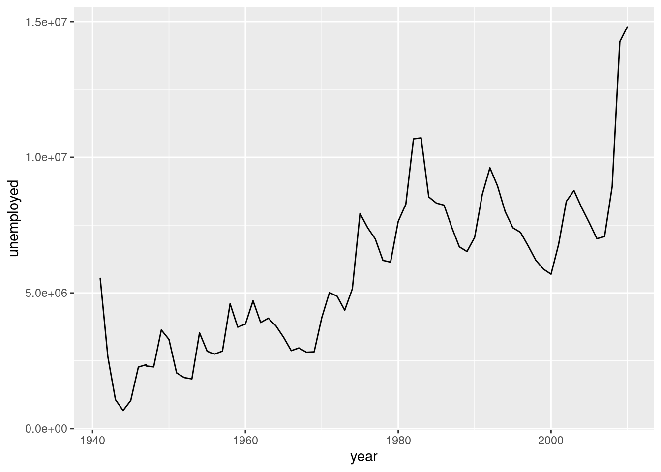
Let’s use the employment dataset and make a simple line plot with year mapped to x and unemployed as y. As stated, line graphs in ggplot are typically made with the help of geom_line(). Let’s make a very simple line graph with the employment dataset, with year on the x axis and unemployed on the y axis. The resulting plot clearly shows how the number of unemployed citizens changes over 70 years.
A simple line graph.
ggplot(employment, aes(x =year, y =unemployed))+geom_line()
Figure F.1: A simple line graph made with geom_line().
The code to make the plot only comprises two lines. During exploratory data analysis, the less typing the better because you want to quickly understand your dataset (likely producing multiple plots like this). However, as good as the default look is, you’ll probably want to make the plots more presentable if you’re going to show them to others. It does take a few more lines of ggplot code (and sometimes some preparatory data transformation, as we did before with dplyr-ing and factor modifications) but the results are worth it!
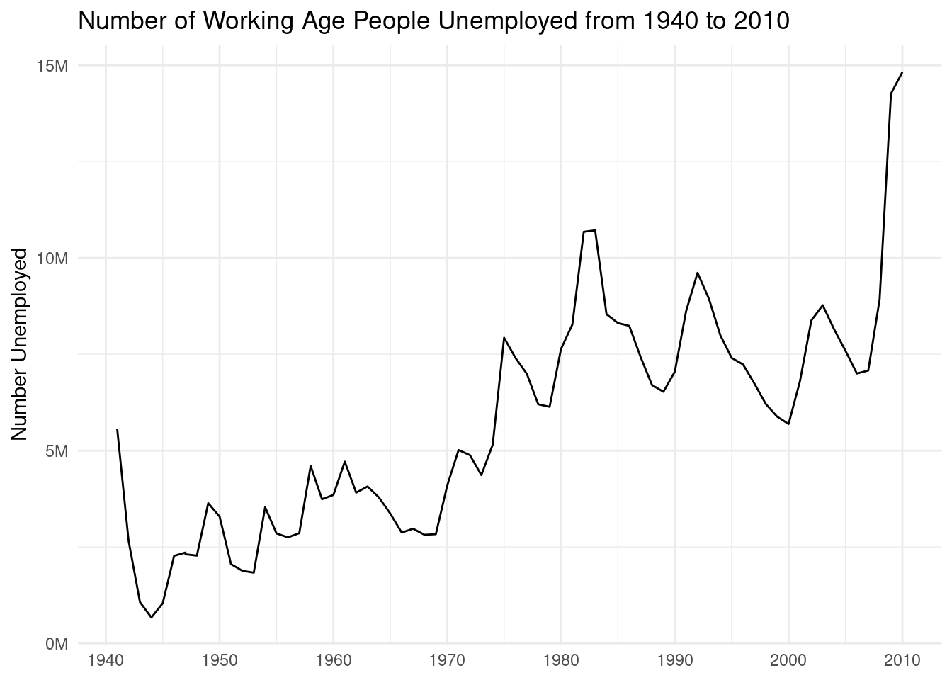
To make the plot look a little nicer, we’ll employ some techniques we’ve used before. In the next code listing, the x- and y-axis scales will be changed with scale_x_continuous() and scale_y_continuous(). With each of those functions, operating on our continuous value axes, we can control the labeling (with the breaks option) and change the number formatting for better readability (with the labels option). The labs() function will be used to label the plot with a title and to modify the y-axis title. Finally, the theme_minimal() function will be applied to reduce the amount of ink used in the plot.
The simple line graph with some styling and customization applied.
ggplot(employment, aes(x =year, y =unemployed))+geom_line()+scale_x_continuous(breaks =seq(1940, 2010, 10))+scale_y_continuous( labels =scales::number_format(suffix ="M", scale =1e-6, accuracy =1.0))+labs( title ="Number of Working Age People Unemployed from 1940 to 2010", x =NULL, y ="Number Unemployed")+theme_minimal()
Figure F.2: A line graph with some styling applied.
The line in the plot is, of course, the same but its environment is a bit more pleasing to the eye. There is higher contrast between the line and the background (thanks to theme_minimal()) and the gridlines are an unobtrusive light gray. The usage of breaks in the x axis allows us to explicitly show years at the head of each decade. The fine-tuning of breaks, like most choices in data visualization, depends on several design factors. The recommendation here is to experiment often with them and fine tune your plots until the look really satisfies you.
The y-axis values were changed from the default scientific notation formatting used for very small or very large numbers. This was done with a combination of scale_y_continuous() and number_format(). The scales package, loaded by default when using library("tidyverse"), contains many useful functions for transforming numerical values, of which number_format() is but one (we’ll use others later in this section). Because the values in the y axis are large, it makes sense to reduce their visual size by scaling and applying a suffix (e.g., 5000000 is transformed to 5M, where M here stands for million). That was done by using the suffix and scale options. With accuracy set to 1.0, we don’t get decimal values (but we would if we used 1.1 instead).
F.1.2 Using geom_line() and geom_point()
The ggplot package allows us to layer several geoms together, and the order in which we call the different geoms determines the stacking order (those called first are lower in the stack). Let’s endeavor to combine geom_line() with geom_point() and, in doing so, we’ll get a line combined with data markers.
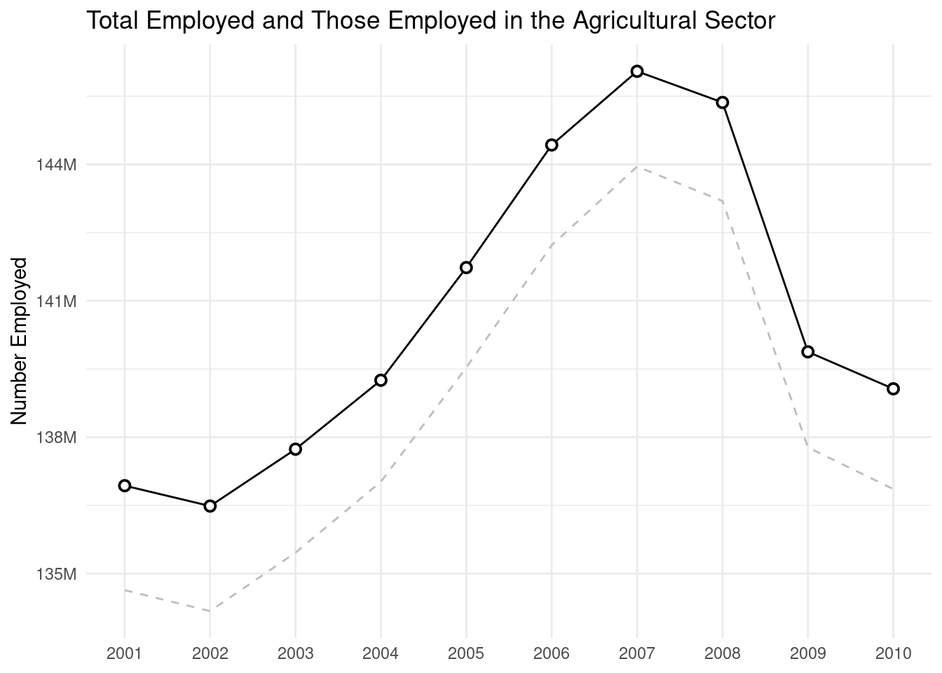
First, let’s get a subset of the employment data using dplyr’s slice_tail() function (it gets the last n rows of a table). The transformed dataset, named employ_recent, is now used to make a new line plot. The key difference here is that we will make two different lines: (1) a solid line using values in the employed column, with circular data points overlaid on top of that line, and (2) a dashed line using values in the nonagriculture column. The line with styled points is made possible with a geom_point() statement called afterward, taking advantage of the layering that ggplot provides.
A line graph with two lines that track closely to each other.
employ_recent<-employment|>slice_tail(n =10)ggplot(employ_recent, aes(x =year, y =employed))+geom_line()+geom_point(size =2, shape =21, fill ="white", stroke =1)+geom_line(aes(x =year, y =nonagriculture), linetype ="dashed", color ="gray")+scale_x_continuous(breaks =seq(2000, 2010, 1), minor_breaks =NULL)+scale_y_continuous( labels =scales::number_format(suffix ="M", scale =1e-6, accuracy =1.0))+labs( title ="Total Employed and Those Employed in the Agricultural Sector", x =NULL, y ="Number Employed")+theme_minimal()
Figure F.3: A line graph consisting of two lines in separate layers.
One thing we tend to miss out on when using separate columns is the automatic drawing of legends. This is a prime reason for using tidy datasets in ggplot. As we’ve done before, manipulation of the data with tidyr’s pivot_longer() is key to making this possible. For the next plot, the transformed dataset employ_recent_tidy was made by selecting a subset of that table’s columns, slicing to get the last 10 rows (i.e., the most recent years of the data), and using pivot_longer() to create a column of values (n) and a column of value types (type). Oh, one more thing, we also got forcats in on the action by releveling the type factor with fct_relevel() (in order of the largest to the smallest values: "population", then "employed", then "unemployed"). We worked on setting factor levels where appropriate so that the order of legend labels is defined.
Making a smaller, tidier version of the employment dataset with tidyr's pivot_longer() function.
# A tibble: 30 × 3
    year type               n
   <int> <fct>          <int>
 1  2001 population 215092000
 2  2001 employed   136933000
 3  2001 unemployed   6801000
 4  2002 population 217570000
 5  2002 employed   136485000
 6  2002 unemployed   8378000
 7  2003 population 221168000
 8  2003 employed   137736000
 9  2003 unemployed   8774000
10  2004 population 223357000
# ℹ 20 more rows
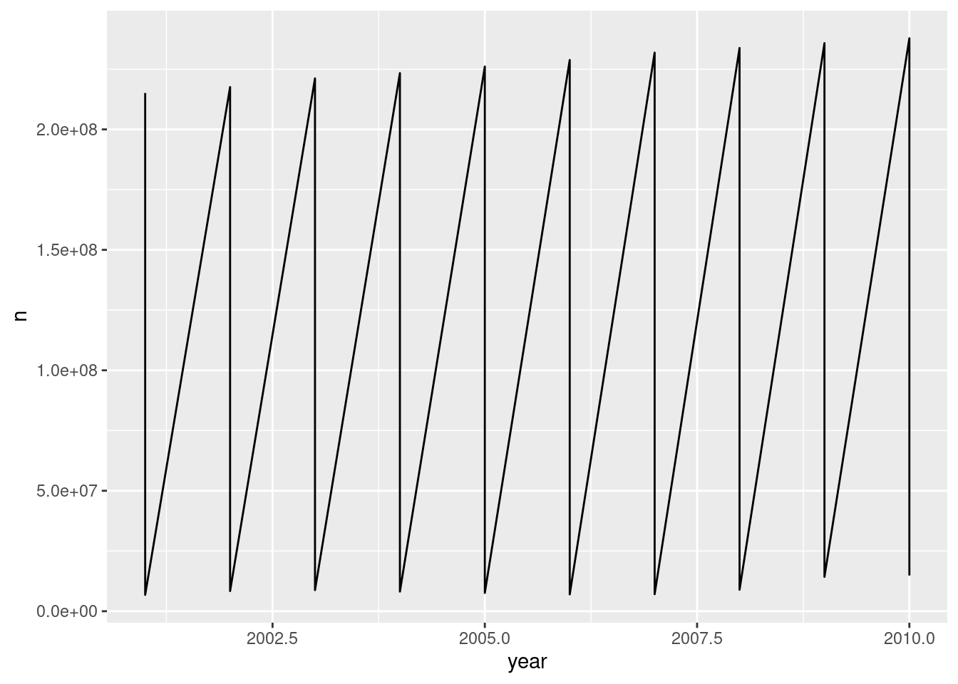
Using a tidy dataset is great but we have to be mindful that a ggplot aesthetic needs to be chosen. Here’s a common example is where we might go wrong: setting only the x and y aesthetics for geom_line(). The plot looks like it has a sawtooth pattern because it’s tracing a line between all points (and they belong to different data series). This happens easily—it can happen to you!—but at least it’s obvious what is happening. And, of course, we have a solution for this coming up soon.
A common pitfall when making line graphs with tidy datasets: a sawtooth pattern.
ggplot(employ_recent_tidy, aes(x =year, y =n))+geom_line()
Figure F.4: A failed attempt at making a line graph with a tidy dataset.
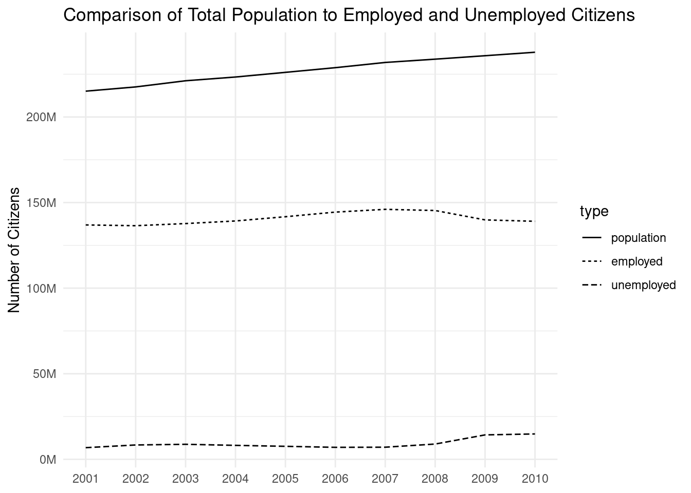
The remedy here is to map the type column to an aesthetic. The aesthetic can be linetype or color and, in the following code listing, we’ve chosen to use linetype. All of the other stylistic choices are in here (making the plot look much better than the previous) and notice that the legend is drawn without even asking for it. Plus, the ordering of labels makes logical sense (they are ordered in the same way they appear in the plot). Basically, the forcats work done previously has paid off, because we didn’t leave this ordering up to chance.
Mapping the linetype aesthetic to the type variable of employ_recent_tidy gives us three separate lines in a single geom_line() call.
ggplot(employ_recent_tidy)+geom_line(aes(x =year, y =n, linetype =type))+scale_x_continuous(breaks =seq(2000, 2010, 1), minor_breaks =NULL)+scale_y_continuous( labels =scales::number_format(suffix ="M", scale =1e-6, accuracy =1.0))+labs( title ="Comparison of Total Population to Employed and Unemployed Citizens", x =NULL, y ="Number of Citizens")+theme_minimal()
Figure F.5: A line graph that uses tidy data and and a suitable selection of aesthetics.
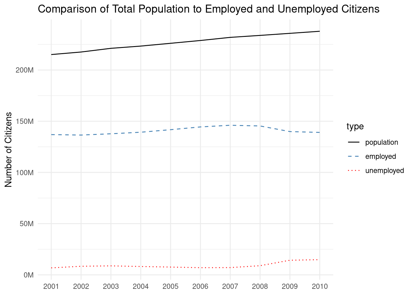
While the line graph looks pretty good, we’re still not satisfied. We want color. We want to change the line styles. We can do it! The ggplot functions you need are scale_color_manual() and scale_linetype_manual(). Within each of those, we use the values argument to pass in a vector colors or line types. The length of the vector depends on the number of factor levels and the order depends on the order of, again, factor levels (can’t say it enough: our work with factor levels has really been worth it). In the next code listing, the two relevant statements are included just after the geom_line() call. The line types used are the of the most common variety, but we made sure to use them in order of decreasing amount of ink ("solid", then "dashed", and then "dotted").
Manually providing linetypes and colors to the three lines is made possible with scale_linetype_manual() and scale_color_manual().
ggplot(employ_recent_tidy)+geom_line(aes(x =year, y =n, linetype =type, color =type))+scale_linetype_manual(values =c("solid", "dashed", "dotted"))+scale_color_manual(values =c("black", "steelblue", "red"))+scale_x_continuous(breaks =seq(2000, 2010, 1), minor_breaks =NULL)+scale_y_continuous( labels =scales::number_format(suffix ="M", scale =1e-6, accuracy =1.0))+labs( title ="Comparison of Total Population to Employed and Unemployed Citizens", x =NULL, y ="Number of Citizens")+theme_minimal()
Figure F.6: A line graph with customized line types and colors.
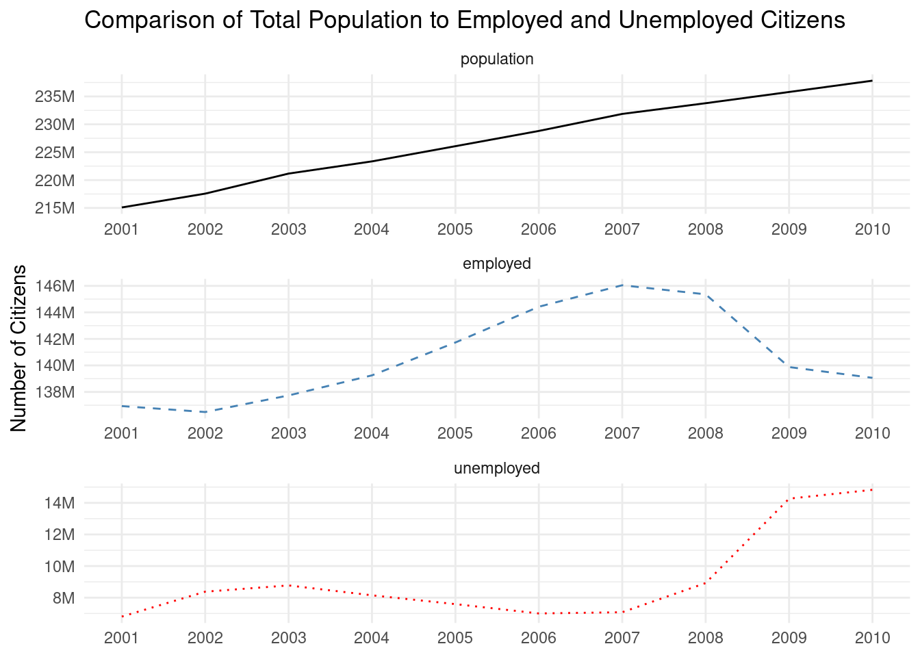
The plot has only subtly changed but all the little details can make a big difference in the end. Something that is striking is that there are large amounts of space between the individual lines. This forces the eye to sweep across all this unused space just to compare the differences between the lines. One strategy is to put the different lines into their own subplots, or facets, and adapt the y-axis scale in each facet to the range of y values (this is otherwise known as using free scales). This is shown next with the use of a facet_wrap() statement, having the scales = "free" option. Because each facet comes with a label, we actually don’t need the legend anymore (it would contain redundant information). It is removed by using theme(legend.position = "none").
Faceting the three lines is possible with facet_wrap() and the legend is probably unnecessary in this arrangement (it's been removed).
ggplot(employ_recent_tidy)+geom_line(aes(x =year, y =n, linetype =type, color =type))+scale_linetype_manual(values =c("solid", "dashed", "dotted"))+scale_color_manual(values =c("black", "steelblue", "red"))+scale_x_continuous(breaks =seq(2000, 2010, 1), minor_breaks =NULL)+scale_y_continuous( labels =scales::number_format(suffix ="M", scale =1e-6, accuracy =1.0))+facet_wrap(vars(type), ncol =1, scales ="free")+labs( title ="Comparison of Total Population to Employed and Unemployed Citizens", x =NULL, y ="Number of Citizens")+theme_minimal()+theme(legend.position ="none")
Figure F.7: A faceted line graph.
Using free scales should only be done with careful consideration. The ggplot default of joint scales in facet_wrap() and facet_grid() is very well chosen and it aids in comparing values across facets without misleading the reader. However, there may be times when the variation in y within some facets simply cannot be seen (this is for data series that are comparatively smaller in magnitude) and using free y scales mitigates this.
The plot concludes our mini-series of line graphs made with the employment dataset. After several iterations, it does look more presentable. Certainly, there are more things that can be done to make the plot even better, but we’ll explore such techniques in upcoming plots.
F.1.3 Using geom_area() to make a line graph
We’ve already combined geom_line() with geom_point() to make a line graph. What will we think of next? Why not use geom_area()? Turns out, it can look pretty good, letting us make line graphs with the area below the line filled in. And, with a carefully considered set of styling options, it can look wonderful.
For the upcoming examples in this section, we’ll use the included-in-dspatternsrainfall dataset. Each row of rainfall is a year of total rainfall amounts in different seven different cities. A glimpse() of the data is given in the following code listing, where we quickly see that the dataset has 8 columns and 25 rows (the range of years is from 1995 to 2019).
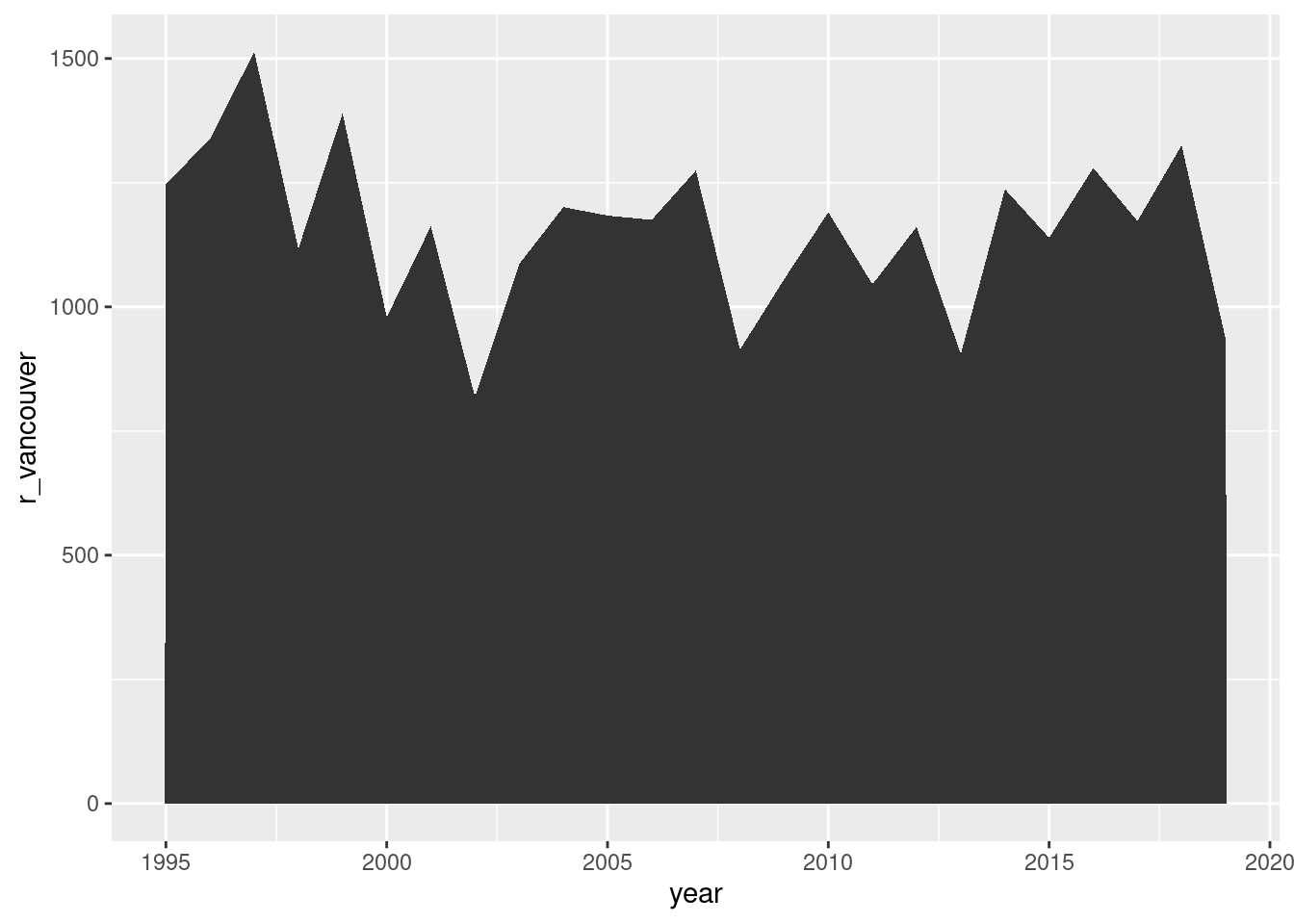
Let’s start with a basic plot, as we often do. The aesthetic mappings required are x and y, so we’ll map the year and r_vancouver columns to those. The geom_area() function will be used without any additional styling options.
A simple line plot with a filled area can be made by use of geom_area().
ggplot(rainfall, aes(x =year, y =r_vancouver))+geom_area()
Figure F.8: A simple line graph made with geom_area().
It doesn’t look like much, but it didn’t take that much to produce either. We can see that the distinctive top portion of the area is the line that traces through the data. An interesting aspect of the geom_area() function is that is has a color aesthetic that controls the color of the line segment representing the data (which doesn’t include the bounding lines of fill area). There is, of course, a fill option and we’ll emphasize the line color and deemphasize the fill with just a few carefully chosen parameters:
It's more visually satisfying to apply some styles in geom_area() like a line color, a fill color, and some transparency.
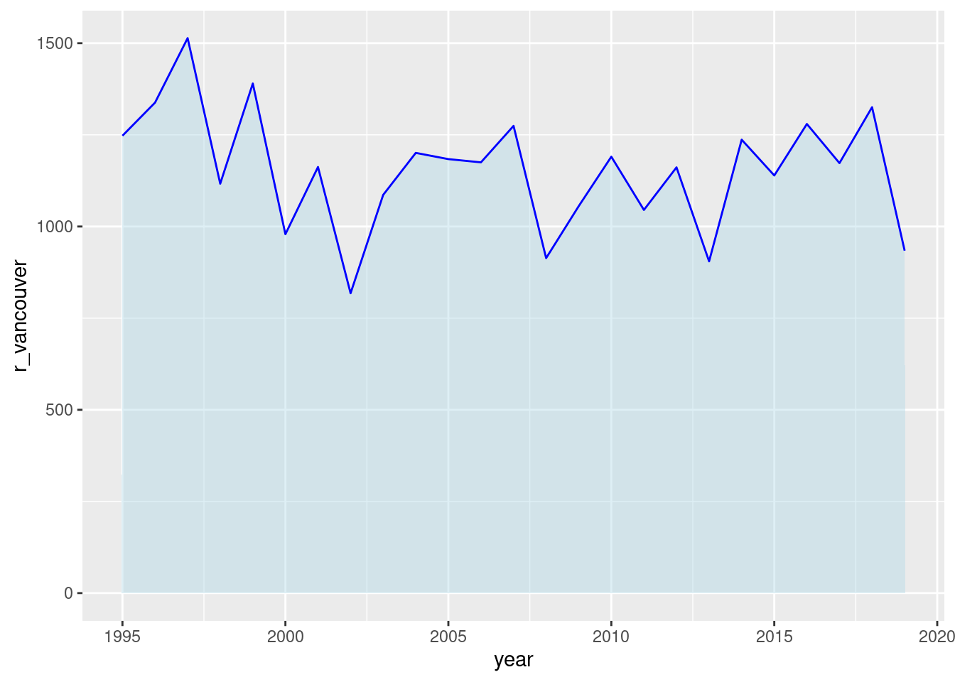
ggplot(rainfall, aes(x =year, y =r_vancouver))+geom_area(color ="blue", fill ="lightblue", alpha =0.4)
Figure F.9: A line graph made with geom_area() and a minimum of customization.
Three constant aesthetic values were used in geom_area(): color (for the color of the line, chosen as "blue"), fill (chosen as a lighter color: "lightblue"), and alpha (which controls the transparency of the fill only). This was enough to bring back the look of a line graph, with the advantage of a filled area below the line.
The use of an underlying area is interesting in this application because it visually emphasizes the difference between lots of rainfall and very little rainfall (since the 0 value of the y axis represents a hard limit: no rain).
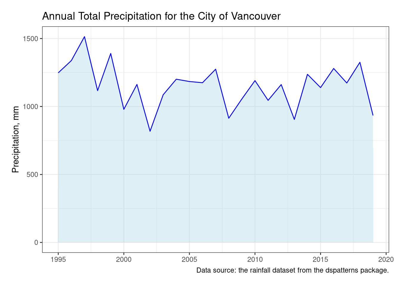
To make this plot presentation-ready, three more statements will be used: labs(), theme_bw(), and theme(). The use of labs() is apparent in the plot: we get a title, a caption, and modified axis labels (removing “year” since it’s obvious the x-axis values are years). The theme offered up by theme_bw() gives us something close to theme_minimal() albeit with a enclosing box on the plot panel. Using theme() allows us to set a huge number of styling options but here we enlarged the plot.margin by 15 pts on each side to give the plot a bit more breathing room (and to avoid having the last x-axis label cut off by the default 5 pt margin).
To complete the look of a line plot with an associated area, a ggplot theme is applied (theme_bw()), and useful labels (like a title and a caption) are paid attention to.
ggplot(rainfall, aes(x =year, y =r_vancouver))+geom_area(color ="blue", fill ="lightblue", alpha =0.4)+labs( title ="Annual Total Precipitation for the City of Vancouver", caption ="Data source: the rainfall dataset from the dspatterns package.", x =NULL, y ="Precipitation, mm")+theme_bw()+theme(plot.margin =unit(c(15, 15, 15, 15), "pt"))
Figure F.10: A fully customized line graph made with geom_area().
The finalized line graph looks presentable. It’s a viable alternative to a more plain line graph generated by geom_line(). The use of color is more visually interesting and it’s furthermore possible to use multiple data series to interesting effect.
F.2 Working with Bar Plots
A bar plot is a common chart type for graphing categorical data or data sorted into groups. It’s usually made up of multiple rectangles aligned to a common baseline. The length of each bar is proportional to the value it represents—in other words, in a bar chart, the data is encoded by length. Our eyes are very good at comparing lengths when objects are aligned, making this graph easy to interpret—just one reason bar charts are often seen.
Our eyes are typically first drawn to base of the plot and then scan towards the end of each bar. We measure the lengths relative to both the baseline and the other bars, so it’s a straightforward process to identify the smallest or the largest bar. We can also see the negative space between varying heights of bars to compare the incremental difference between them.
Not only are these graphs easy to read, but they are also widely recognized. We’ve already done some work in previous sections with horizontal or vertical bar plots, but we’ll go even further here, closely looking at clustered bar plots and stacked bar plots. Turns out that the main difference between those two types is how the bar segments are dodged.
F.2.1 Vertical Bar Plots
This section serves as a bit of a review and it’s good to start with a basic plot anyway. The rainfall dataset will serve us well here. In the next bit of plotting code we swap out the geom_area() function for the geom_col() function.
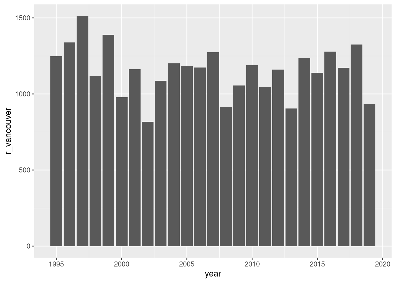
Using geom_col() instead of geom_bar(stat = "identity") to make a simple bar chart of total annual rainfall statistics for Vancouver.
ggplot(rainfall, aes(x =year, y =r_vancouver))+geom_col()
Figure F.11: A simple vertical bar plot.
Previously, we had used geom_bar() with stat = "identity". Why not here? Think of geom_col() as a shortcut for that specialized usage of geom_bar(). The values passed to geom_bar() are directly taken as the length of the bars. Anyway, the plot is quite basic and in its current design, it really doesn’t do anything all that different. There seems to be more value in a bar plot that uses categorical values for the bars (though one could argue that different years could be considered as different categories). In following parts of this section, we’ll move in that direction and try to play to the strength of bar plots: visualizing differences in individual values both within and across groups. The immediate lesson here however is that geom_col() exists and is easier to use than geom_bar() (if your data suits it).
F.2.2 Clustered Bar Plots
Clustered bar plots contain bars that exist in the same plot but are associated with different groups. It can be said that the different groups form different clusters of bars, and, the number of bars in each group doesn’t have to be the same. All of the bars originate from the same axis (i.e., they are not stacked) and some additional spacing or other visual cues to differentiate the groups. We’ll continue to use the rainfall dataset and, in doing so, use more data from it and work toward the best arrangement of bars.
We need to do some tidying work on rainfall. The problem is something we’ve several times before: each row does not represent a single observation (but rather seven observations). No worries, tidyr’s pivot_longer() function will be used to solve this problem. Aside from this very necessary operation, we’ll do two more things: (1) filter() the data to the three most recent years in the dataset (2017–2019), and (2) mutate() the city and year columns to be factors with a specific ordering. This is all done to make the transformed dataset called rainfall_recent_tidy:.
Making a smaller, tidier version of the rainfall dataset with tidyr's pivot_longer() function.
rainfall_recent_tidy<-rainfall|>slice_head(n =3)|>pivot_longer( cols =starts_with("r"), names_to ="city", names_prefix ="r_", values_to ="precip")|>mutate( city =factor(city)|>fct_inorder(), year =factor(year)|>fct_inseq())rainfall_recent_tidy
# A tibble: 21 × 3
   year  city      precip
   <fct> <fct>      <dbl>
 1 2019  vancouver   934.
 2 2019  calgary     317
 3 2019  kenora      566.
 4 2019  toronto     800.
 5 2019  montreal    947.
 6 2019  halifax    1283.
 7 2019  stjohns    1188.
 8 2018  vancouver  1325.
 9 2018  calgary     244
10 2018  kenora      487.
# ℹ 11 more rows
Now that we have two dedicated factor columns (year and city) and one value column (precip), we can make a clustered bar chart. The key to this is choosing which columns to map to x and y and a visual aesthetic (here we’ll use fill). Also, and this is important, the position = "dodge" option must be used in geom_col(). This is what does the clustering (and avoids the stacking). As a first attempt, year will be mapped to x (as before), precip will be mapped to y (similar to before), and city will be mapped to fill (this is new).
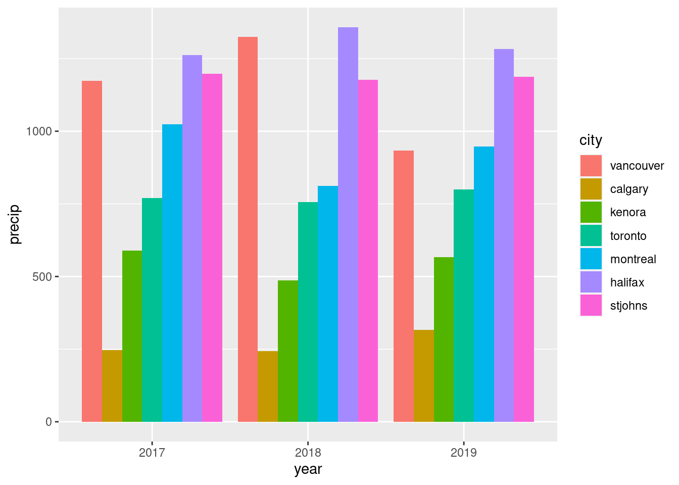
Making a clustered bar chart is now possible with the tidy dataset with city and precip as new variables. Note the use of position = "dodge" to avoid stacking the bars.
ggplot(rainfall_recent_tidy, aes(x =year, y =precip, fill =city))+geom_col(position ="dodge")
Figure F.12: A simple horizontal, clustered bar plot with default colors applied.
The clustered bar plot clearly shows the groupings of the x axis (the years) and the different bars represent the precipitation totals of the different cities. The automatically drawn legend is a definite plus and a side benefit of using tidy data. The question remains however: does this arrangement of groups communicate well? Perhaps city would be a better first order grouping (along the x axis) so that would can better compare rainfall totals each year for each city? If that’s the intention, then it’s an easy modification: swap the city and year variables between the x and fill aesthetics.
Redefinition of the x values as the cities instead of the years, where the fill aesthetic is now mapped to year.
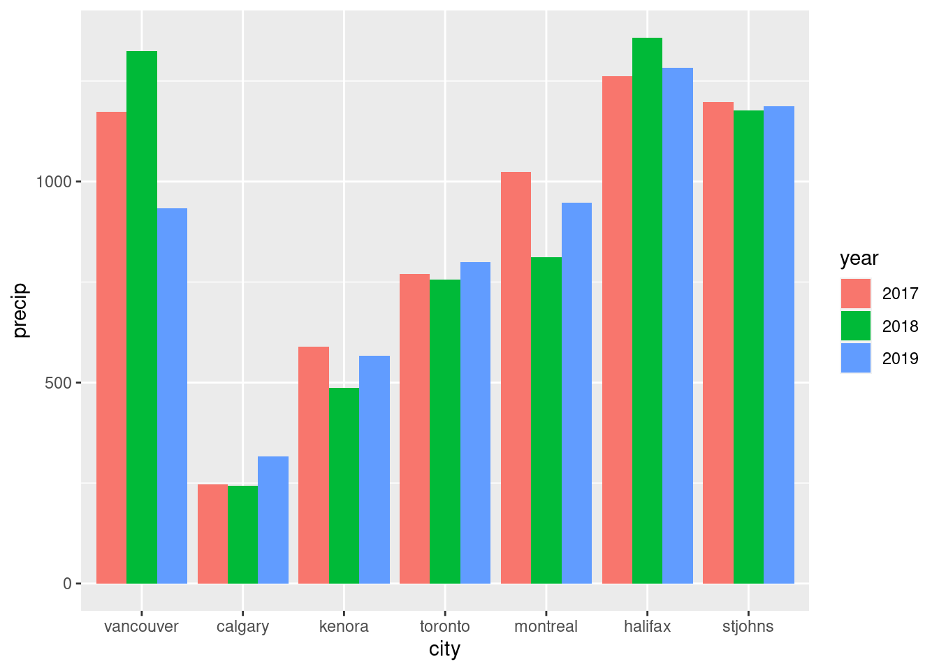
ggplot(rainfall_recent_tidy, aes(x =city, y =precip, fill =year))+geom_col(position ="dodge")
Figure F.13: A clustered bar plot that uses categorical data on the x axis.
Now that the bars are arranged in a manner that better communicates the data, we can focus on making it presentation ready. Notice that in previous rainfall plots, the order of years and of cities (arranged from west to east, as it was in the original rainfall dataset) is maintained thanks to the work in setting factor levels. This is helpful in that we don’t have to manually arrange the values within the ggplot code.
To get to the final version of the plot, we’ll do a great many things:
Increase the amount of space between clusters with geom_col()’s width option.
Use sequential fill colors for bars in each cluster (with scale_fill_brewer()).
Relabel the x-axis labels with correct city names with scale_x_discrete()’s label option.
Ensure that the y-axis spans from 0 to 1500 using coord_cartesian() and ylim.
Directly label the first cluster of bars with year labels (using annotate() three times).
Add a plot title, subtitle, and caption, and, modify the axis titles (all with labs()).
Apply the minimal theme with theme_minimal().
Remove the vertical gridlines by setting panel.grid.major.x to element_blank() in theme().
Remove the legend (legend.position = "none" in theme()).
Move up x-axis labels a little with element_text(vjust = 5) in theme().
It’s a lot of stuff to do (and it’s all done in the upcoming code listing) but the results are definitely worth it because the plot looks ultra-presentable.
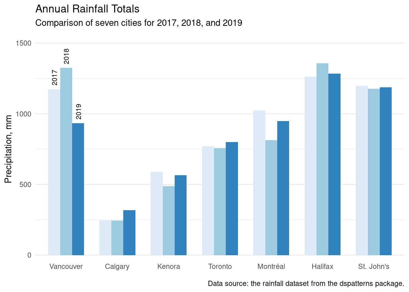
A very presentable version of the previous barplot; there are customizations galore in here (and the extra code is worth it in the end).
ggplot(rainfall_recent_tidy, aes(x =city, y =precip, fill =year))+geom_col(position ="dodge", width =0.7)+scale_fill_brewer("Blues")+scale_x_discrete( labels =c("vancouver"="Vancouver", "calgary"="Calgary","kenora"="Kenora", "toronto"="Toronto","montreal"="Montréal", "halifax"="Halifax","stjohns"="St. John's"))+coord_cartesian(ylim =c(0, 1500))+annotate( geom ="text", x =0.77, y =1200, label ="2017", hjust =0, angle =90, size =3)+annotate( geom ="text", x =1.00, y =1350, label ="2018", hjust =0, angle =90, size =3)+annotate( geom ="text", x =1.24, y =960, label ="2019", hjust =0, angle =90, size =3)+labs( title ="Annual Rainfall Totals", subtitle ="Comparison of seven cities for 2017, 2018, and 2019", caption ="Data source: the rainfall dataset from the dspatterns package.", x =NULL, y ="Precipitation, mm")+theme_minimal()+theme( panel.grid.major.x =element_blank(), legend.position ="none", axis.text.x =element_text(vjust =5))
Figure F.14: A presentation-ready clustered bar plot.
Clustered bar plots, if used effectively, can be useful for comparisons of individual values both within groups and across groups. Getting to a presentation-ready plot of this type is possible with a dozen lines of carefully considered ggplot code.
F.2.3 Stacked Bar Plots
Stacked bar plots take all the bars from a group and stack them up, forming a sort of tower from the individual bars. The interesting thing here is that the arrangement of the component segments can be controlled (as always taking advantage of factors is the best way to accomplish this). When should we use a stacked bar plot? It makes a lot of sense when bar components of part of a whole and the combined length is meaningful. So, stacking up yearly rain totals for a city doesn’t really produce a total we might care about but stacking up the number of residents that live in each city ward seems like a good idea (the length of the stacked bar is the city population and we get a feel for which wards are big, small, or somewhere in the middle.
We’ll turn our attention to German cities for this part of the section We’ve used the german_cities dataset in the last section and it’s well suited for demonstrating the usefulness of stacked bar plots here. Thanks to dplyr’s glimpse(), we can have a second look at this dataset of 4 columns and 79 rows (where each row is a city).
As in the previous set of examples on clustered bar plots, an iterative, stepwise approach will be taken to progress toward the final, presentation-ready or publication-ready plot. We will experience all the heartache that comes with the setup phase of a plot that has promise. Let’s experience the blues from the very first example. We’re starting simple, using geom_col() (no dodging this time), choosing to map the city name to fill. However, the autogenerated legend will be overwhelmingly huge.
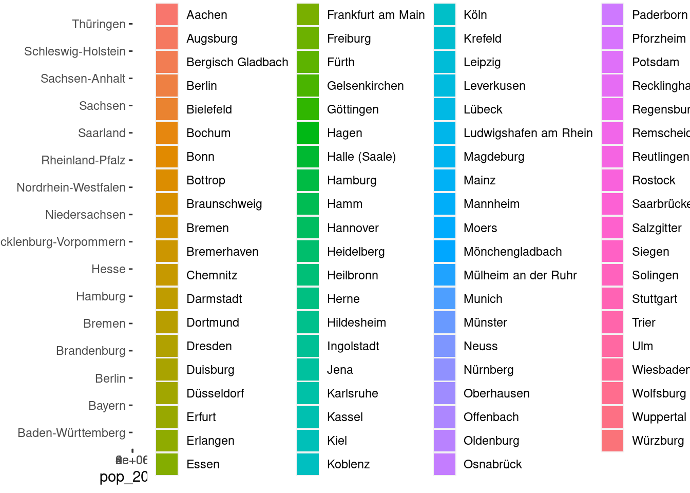
An attempt at a stacked bar plot with the german_cities dataset is an abject failure (the legend is pretty much all we see).
german_cities|>ggplot(aes(x =pop_2015, y =state, fill =name))+geom_col(aes(fill =name))
A failed attempt at a stacked bar plot. The legend is too big.
Really, a legend like the one above is useless. We don’t actually need to know the names of each city in the stacked bars. Maybe knowing the name of largest city in each state is helpful but the plot better serves us if shows us the make-up of large cities across each state. We can ditch the legend by adding theme(legend.position = "none") to the ggplot code. In doing this, we can see plot at full width, which serves as a more reasonable starting point for further improvements.
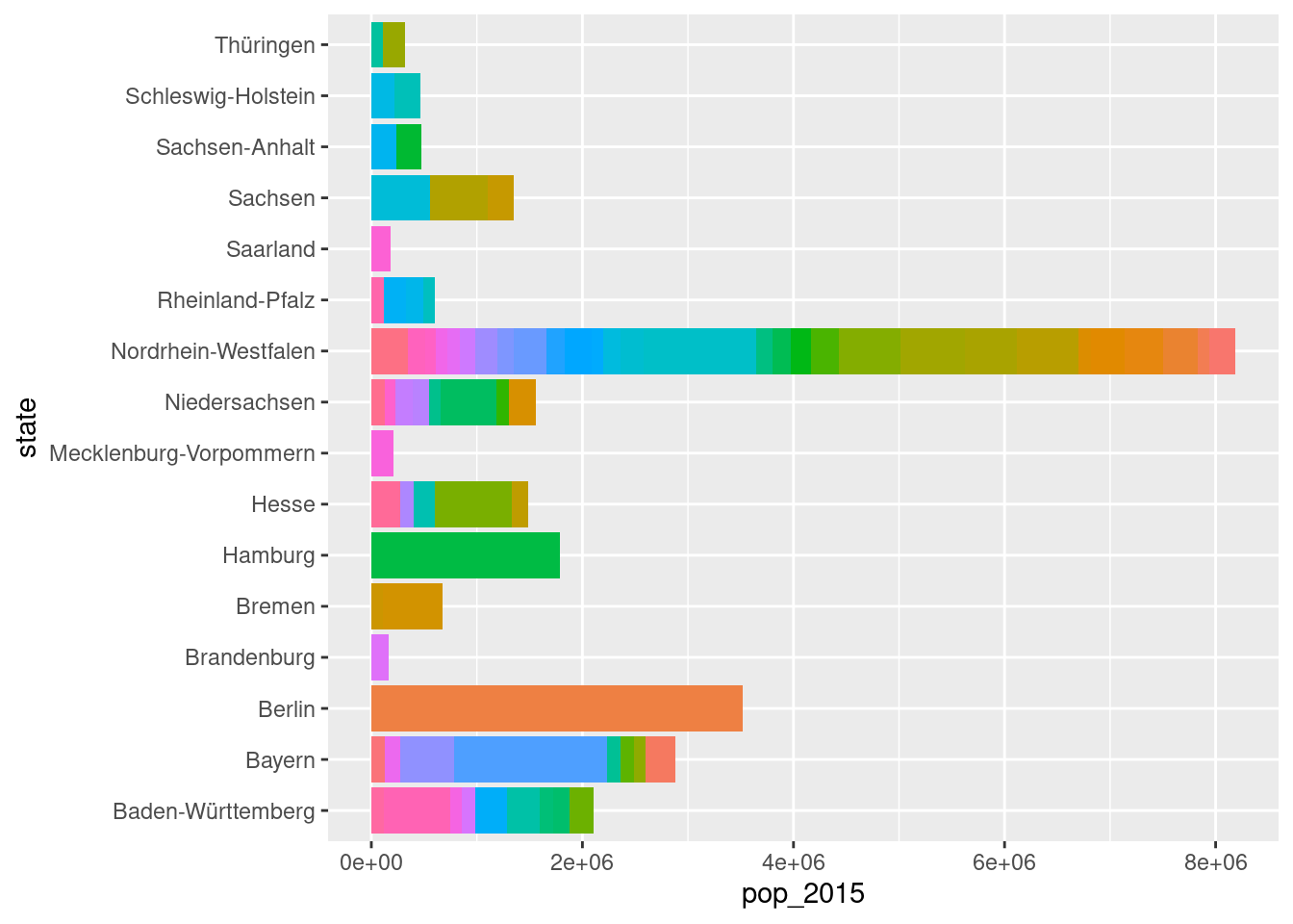
A second attempt at the stacked bar plot now lets us see the plot, and we don't need a legend here anyway.
german_cities|>ggplot(aes(x =pop_2015, y =state, fill =name))+geom_col(aes(fill =name))+theme(legend.position ="none")
A basic stacked bar plot with no legend.
The plot does give us information on the composition of large cities in each state in Germany but it’s far from presentable. The first, glaring problem is the lack of arrangement of the stacked bars. The second problem, and this is less obvious, is that the internal arrangement of bar segments in each stacked bar is not ordered. For this plot, the ordering parameter that should be used is the population (using the populations given in the pop_2015 column of german_cities). The goal is to get stacked bars from large to small running from top to bottom, and, in each stacked bar, large to small bar segments from right to left.
To get this process underway, we need to work on transforming the german_cities dataset. As with the rainfall transformation, we need to have two columns transformed to factor columns and those two columns in german_cities are name and state. First, we need to add a column that has the total population of each state (total_pop). The values in that column will be used to reorder the factor levels of the state column (in a descending manner, with the .desc option set to FALSE). This code lising provides the code and output for this, yielding the transformed dataset called german_cities_totals:
Transforming our german_cities data is required to get a total population by state (total_pop) column and to reorder factor levels (improving the order of bars and the segments within).
german_cities_totals<-german_cities|>group_by(state)|>arrange(desc(pop_2015))|>mutate(total_pop =sum(pop_2015))|>ungroup()|>mutate( state =state|>fct_reorder(total_pop), name =name|>fct_reorder(pop_2015, .desc =TRUE))|>select(-pop_2011)german_cities_totals
# A tibble: 79 × 4
   name              state               pop_2015 total_pop
   <fct>             <fct>                  <int>     <int>
 1 Berlin            Berlin               3520031   3520031
 2 Hamburg           Hamburg              1787408   1787408
 3 Munich            Bayern               1450381   2882013
 4 Köln              Nordrhein-Westfalen  1060582   8190394
 5 Frankfurt am Main Hesse                 732688   1485977
 6 Stuttgart         Baden-Württemberg     623738   2101693
 7 Düsseldorf        Nordrhein-Westfalen   612178   8190394
 8 Dortmund          Nordrhein-Westfalen   586181   8190394
 9 Essen             Nordrhein-Westfalen   582624   8190394
10 Leipzig           Sachsen               560472   1352942
# ℹ 69 more rows
This revised dataset is nearly tidy, but we’ll keep the two population columns (pop_2015 and total_pop) in this table since we’ll later use the total_pop column to help us annotate the stacked bars in the final plot.
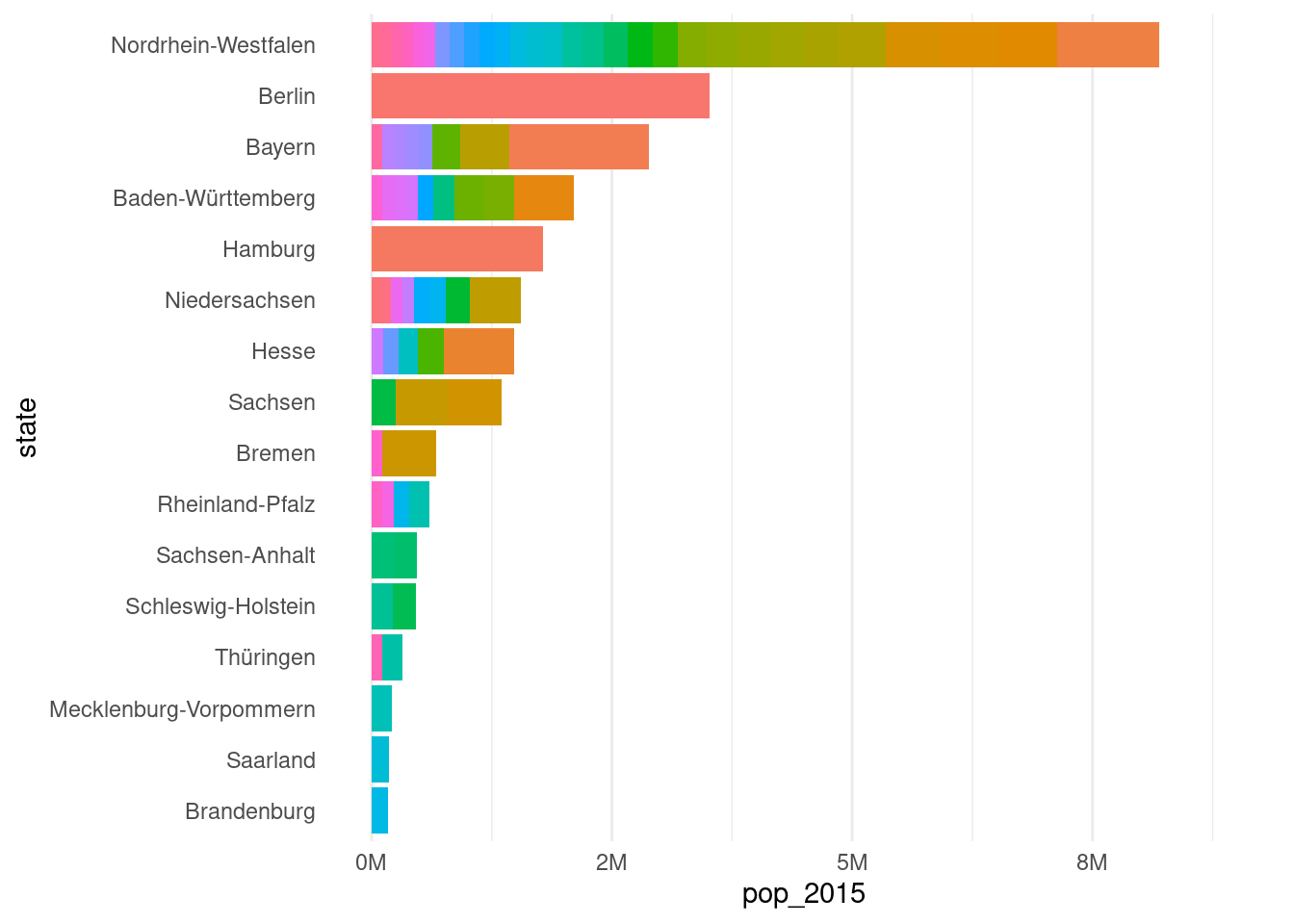
In the third attempt at making the stacked bar plot, we use the german_cities_totals dataset. The aesthetic mappings in aes() remain the same but we do add a few statements to clean up the x-axis labels and apply theme_minimal(). The resulting plot now has the correct ordering of stacked bars and bar segments.
A third attempt at the german_cities stacked bar plot: bars are in descending order, cities are stacked by population (increasing, left to right), and the x-axis labels are more readable.
german_cities_totals|>ggplot(aes(x =pop_2015, y =state, fill =name))+geom_col()+coord_cartesian(xlim =c(0, 9E6))+scale_x_continuous( labels =scales::number_format(suffix ="M", scale =1e-6, accuracy =1.0))+theme_minimal()+theme( legend.position ="none", panel.grid.major.y =element_blank())
A stacked bar plot with bars ordered by length.
This is progress! The plot is structurally how we want it. Now, the remaining task is to make this plot shine with customizations attuned to presentation. In practice, you can take this as far as you want to. For the most part, if you can think of something useful to add, it is possible, but you have to discover a method for doing so. Here, we’ll want to do a few things:
Make each component of every bar clearly distinguishable with a white outline by setting the constant aesthetic color to "white".
Use of a monochromatic color scale for each stacked bar component with scale_fill_grey().
To the right of each stacked bar, provide the name the largest city in the state with geom_text().
To the left of each bar (and to the right of the state name), add a label showing the number of cities in each stacked bar (again, with geom_text()).
Ensure that there are vertical axis lines at every 1 million residents by setting breaks in scale_x_continuous(); exclude minor axis lines with minor_breaks = NULL.
Make the vertical line where the bars originate a bit more prominent by using geom_vline().
Add a plot title, a subtitle, and a caption; remove the x- and y-axis titles (all with labs()).
Push the plot title and subtitle to the left edge of the plot with plot.title.position = "plot" and plot.caption.position = "plot" in theme().
These requirements are all possible but first we need an extra data table that contains the largest city in each state, the total population of each state, and the number of cities in each state. We can derive this table starting from german_cities_totals. This is completely a dplyr exercise where we: (1) group_by() the state, (2) arrange() each group by descending population, (3) get a total column n which counts of the number of cities in each group/state (through mutate(n = n())), (4) slice() to get the first (largest) city in each group/state, and (5) remove the unneeded pop_2015 column (through select()). Here’s the the code and the output for the newly created german_cities_largest table.
In order to directly label the largest cities in each of the bars, we need a separate dataset of just those dominant cities for geom_text().
# A tibble: 16 × 4
# Groups:   state [16]
   name              state                  total_pop     n
   <fct>             <fct>                      <int> <int>
 1 Potsdam           Brandenburg               167745     1
 2 Saarbrücken       Saarland                  178151     1
 3 Rostock           Mecklenburg-Vorpommern    206011     1
 4 Erfurt            Thüringen                 319645     2
 5 Kiel              Schleswig-Holstein        462559     2
 6 Halle (Saale)     Sachsen-Anhalt            472714     2
 7 Mainz             Rheinland-Pfalz           601997     4
 8 Bremen            Bremen                    671489     2
 9 Leipzig           Sachsen                  1352942     3
10 Frankfurt am Main Hesse                    1485977     5
11 Hannover          Niedersachsen            1555465     8
12 Hamburg           Hamburg                  1787408     1
13 Stuttgart         Baden-Württemberg        2101693     9
14 Munich            Bayern                   2882013     8
15 Berlin            Berlin                   3520031     1
16 Köln              Nordrhein-Westfalen      8190394    29
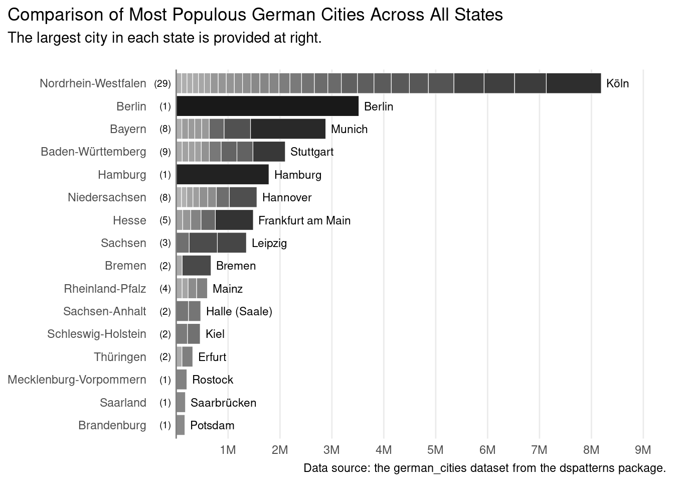
Now that we have the german_cities_largest table, we can address requirements (3) and (4), which both involve adding labels through the geom_text() function. Here’s the finalized ggplot code:
The final stacked bar plot, which gives useful information on large cities within each German state through clearly defined bar segments and helpful annotations.
german_cities_totals|>ggplot(aes(x =pop_2015, y =state, fill =name))+geom_col(color ="white", linewidth =0.2)+scale_fill_grey(end =0.7, start =0.1)+geom_text( data =german_cities_largest,aes(y =state, x =total_pop, label =name), size =3, hjust =0, nudge_x =1e5)+geom_text( data =german_cities_largest,aes(y =state, x =0, label =paste0("(", n, ")")), size =2.5, hjust =1, nudge_x =-1e5)+coord_cartesian(xlim =c(0, 9E6))+scale_x_continuous( labels =scales::number_format(suffix ="M", scale =1e-6, accuracy =1.0), breaks =seq(1e6, 9e6, 1e6), minor_breaks =NULL)+geom_vline(xintercept =0, color ="gray50")+labs( title ="Comparison of Most Populous German Cities Across All States ", subtitle ="The largest city in each state is provided at right.\n", caption ="Data source: the german_cities dataset from the dspatterns package.", x =NULL, y =NULL)+theme_minimal()+theme( legend.position ="none", panel.grid.major.y =element_blank(), plot.title.position ="plot", plot.caption.position ="plot")
A stacked bar plot that is complete and presentation ready.
There’s a lot of code needed to make this plot! Worth some discussion here is the use of geom_text(). Like all geoms, it requires data but using the german_cities_totals data (passed to ggplot() and used by geom_col()) wouldn’t work because it contains too many rows. We need as many rows as there are states (or stacked bars), so that’s the rationale for creating a secondary dataset.
Now let’s look at some of the details regarding our use of geom_text(). The scale that x uses in geom_text() is the population scale, and the total_pop column (mapped to x) gets us to the end of each stacked bar. However, by default, text is rendered by geom_text() with a centered justification. So, half of the text (the left side) would land on the bar and that’s really not a good look. Instead, we need left justification for text and that setting is hjust = 0 (0.5 is center, and 1 is right). In the first geom_text() call, we do justify the text to the left, then, we nudge it a bit to the right via nudge_x = 1e5 (the value is still using the x/population scale). The only other tweak is the size option, which refers to the size of the text. I found that using size = 3 made the text legible but not overly obtrusive.
The second geom_text() call puts the number of cities in parentheses. The label option allows for an R expression, which is great because we can use paste0() to generate strings using data and string literals (i.e., the surrounding parentheses). Aside from the pasting trick, this geom_text() statement tries to do the reverse of the previous geom_text() call, nudging the text to the left of the x = 0 point and right justifying that text (with hjust = 1). There was some setup required for using geom_text() but it’s a lot more efficient than using annotate() dozens of times (which is never worth it).
For a plot like this, it does really take some time to get everything set up just so. And, it can be a matter of making the tradeoff between time and quality. But with enough tricks up your sleeve you can routinely rattle off plots just as good. The plot does convey that some states are composed of lots of small to mid-size cities (Nordrhein-Westfalen having the well-known, densely populated Rhine-Ruhr megacity) to states encompassing a city (Berlin, Hamburg). It being stacked gives us a picture of the combined population of large cities in each state, which is an interesting metric for comparison.
F.3 Summary
A line graph is used to show a series of data points connected by straight line segments; it can be made in ggplot using at least three different approaches: (1) with geom_line(), (2) with geom_line() and geom_point() (to show points along the line), or (3) with geom_area() (best done with additional styling that emphasizes the line portion).
Horizontal or vertical bar plots can be made in ggplot with geom_col(), mapping categorical values and bar length values as appropriate to the x and y aesthetics.
Clustered bar plots can be made with geom_col() by using position = "dodge" and by supplying three aesthetics: the mandatory x and y (for the major groupings and the bar lengths) and a third one (of which color is recommended).
A stacked bar plot is useful when the overall lengths of the stacked bars are meaningful; they are made with geom_col() much in the same way as clustered bar plots except that we don’t use position = "dodge" for this application.
We can make a plot more presentation ready by adding/modifying labels (with labs()), setting a predefined theme (e.g., theme_minimal() or theme_bw()), modifying one or more theme elements (with the huge amount of options in theme()), using plot annotations (with geom_text() and annotate()), modifying axis breaks (by using breaks in the scale_x_continuous() and scale_y_continuous() functions), or setting custom color palettes (e.g., scale_fill_brewer(), scale_fill_grey(), etc.).
To help ggplot make better plots (with automatic legends and a sensible ordering of plot elements), we often need to transform the data with functions from dplyr (e.g., select(), filter(), mutate(), group_by(), arrange(), etc.), tidyr (pivot_longer()), and forcats (any relevant fct_*() function for setting/modifying factor levels).